SciLifeLab Workshop 2025

Download Tutorial Dataset

You can download a tutorial dataset of urate oxidase here. (ca. 60 GB)

Open Dataset

To save some time for the import, I already converted the datasets from Velox/.emd format to HDF5. Each dataset folder contains an .h5 file and .ini file. Start by adding the .ini files to the workspace.

Note: You can see that the file names end on a timestamp. This timestamp gets added to the file name upon importing. You can import the same file again if you want to try processing with different settings - the timestamp ensures you will not accidentally overwrite your previous results and keeps a paper trail of what you tried.

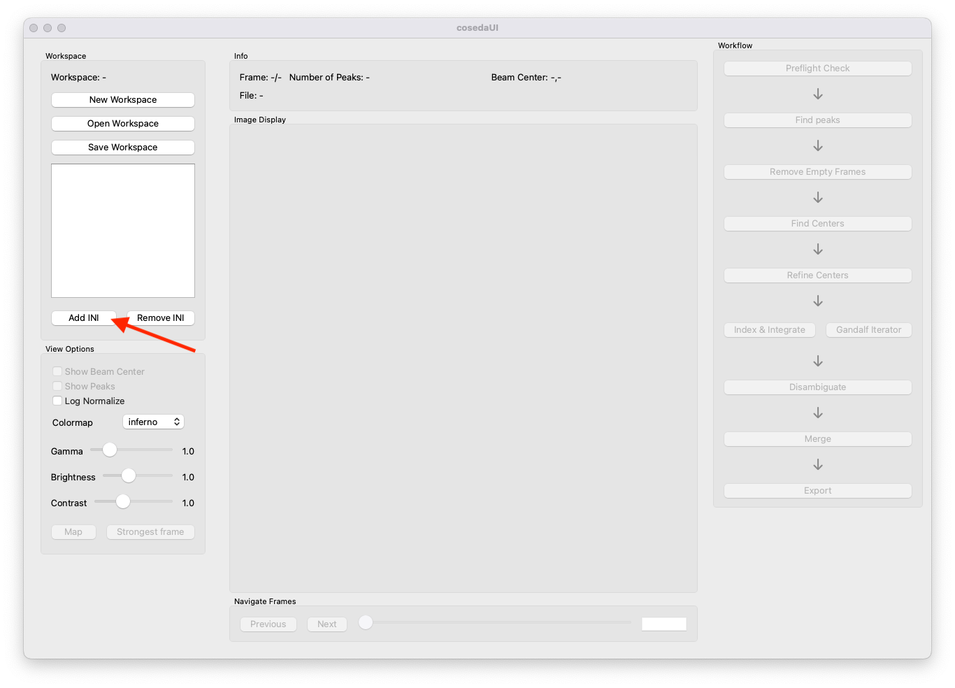
Once you added all of them, save the workspace. To keep things tidy, the best way is to place it aside the dataset folders.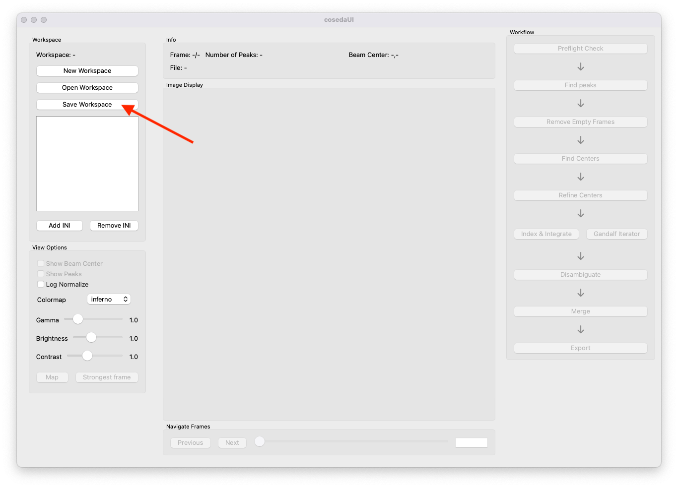

If saving was successful, you should see the name of the workspace here: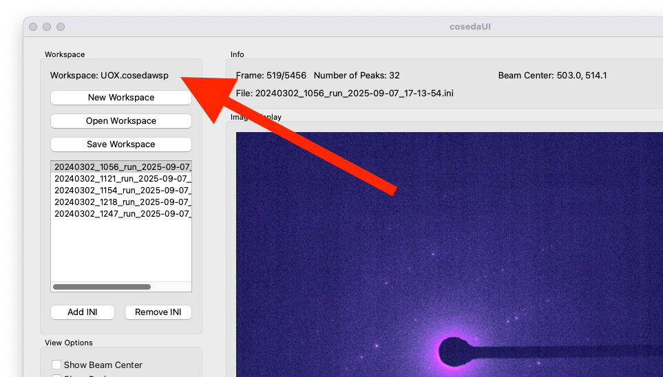

You can use the view options to adjust the image to improve the visibility of features you’re interested in. This is only for preview and does not change the file itself.

Preflight Check

The .ini file is the heart of the processing. It looks somewhat like this:

\[Paths\]
framepath = entry/data/images

\[AcquisitionDetails\]
camera_length_correction = 1
acceleration_voltage = 300000
resolution_width = 4096
resolution_height = 4096
binning_width = 4
binning_height = 4
camera_length = 2.3698
adu_per_photon = 5`

\[Parameters\]

You can see that there are different sections for paths, metadata and processing parameters.

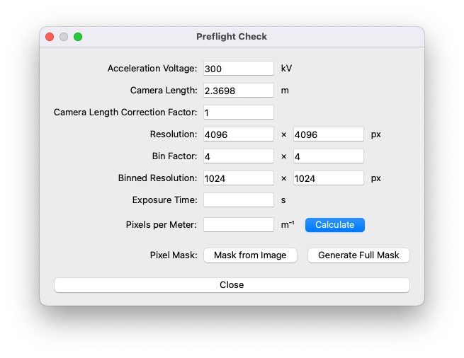
When we import a new file, the import script will try to fetch as much metadata as possible from the original file. Unfortunately sometimes some of them are missing. The Preflight Check ensures helps you to check and complete all metadata essential for the processing. Oops, seems like I accidentally deleted the physical pixels size - please add it again! The data was collected on a Ceta-D camera using bin factor 4.

Find Peaks

Currently we only have peakfinder8 implemented in the (more will come in the future), but it turned out to work well with Ceta-D data. You can experiment with the parameters to see what works best for your data. Enable the live preview and shuffle through some frames. Try to find settings that cover the whole spectrum from intense to weak peaks, while preventing to wrongly identify noise or background as peaks.

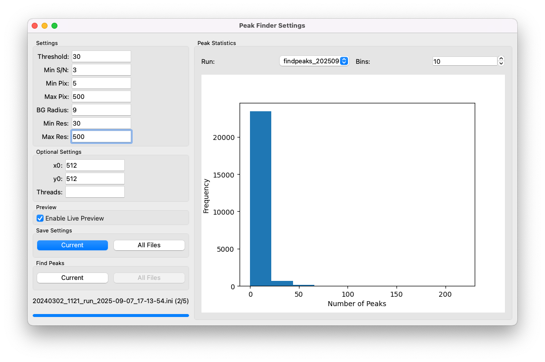
If you are lost, here are some good staring points for the UOX dataset:

• threshold: 30

• minimum S/N: 3.0

• minimum pixel count: 5 px

• maximum pixel count: 500 px

• local background radius: 9 px

• minimum resolution: 30 px

• maximum resolution: 500 px

• x0: 512

• y0: 512

Remove Empty Frames

Dependent on how dense you pack your grid, in continuous serialED experiments you will collect a lot of empty frames when you move in between the crystals. If you collect data with a e.g., this data does not get sorted out automatically. As they do not contain any valuable information, we can safely discard the empty frames. After peak finding is finished, the Remove Empty Frames button in the workflow tree should be activated.

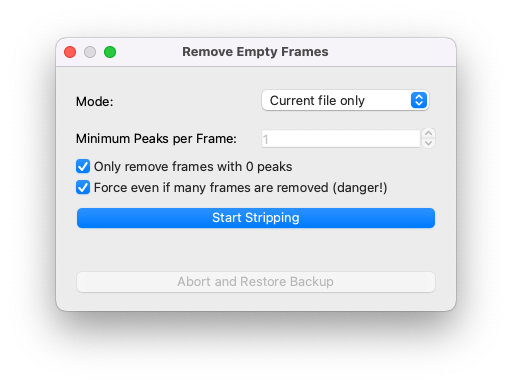
You can set a threshold in this window, all frames in the dataset containing less peaks than the threshold will be deleted. This can drastically reduce the amount of disk space required. Our UOX dataset for example will have about 20% of its original size, if you just remove empty frames. Even if you do not intend to remove any data, it is still recommended to run this function, as it repacks and chunks your HDF5 file, which improves read and write times. This will noticeably speed up your processing later. Rewriting your file might take a little while if your hard drive is not the fastest. Now is a good time for Fika.

Note: In case your dataset contains a high share of empty frames, the function will refuse to run. This is meant to prevent you from deleting too much data by accident. If you are sure your peak finder settings gave you sensible results, tick the force box and try to run it again.

Find Centers

A major challenge when collecting single-shot diffraction patterns on a TEM (compared to XFEL or Synchrotron), is that the beam is shaped and steered by electromagnetic lenses and deflectors. Small instabilities (e.g., in lens currents) can result in significant fluctuations of the beam position. However, for successful indexing, it is crucial to have exact knowledge of the beam position. In COSEDA we implemented a two step process, consisting of beam center finding and successive refinement. There reliable method based on clustering of Friedel pair midpoints. This method is preferred for data with lots of reflections per frame. There is also an intensity based one, but it is still in experimental state. Since our UOX data was collected with a beamstop (=we cannot see the primary beam), we can only use the Friedel pair method.

We start by separating our dataset in at least 4 subsets. For each of this subset, we accumulate the midpoints of all Friedel pairs using unsupervised clustering. The batch centers are then used to interpolate centers for each individual frame. This will take care of the linear drift occurring during the data collection.

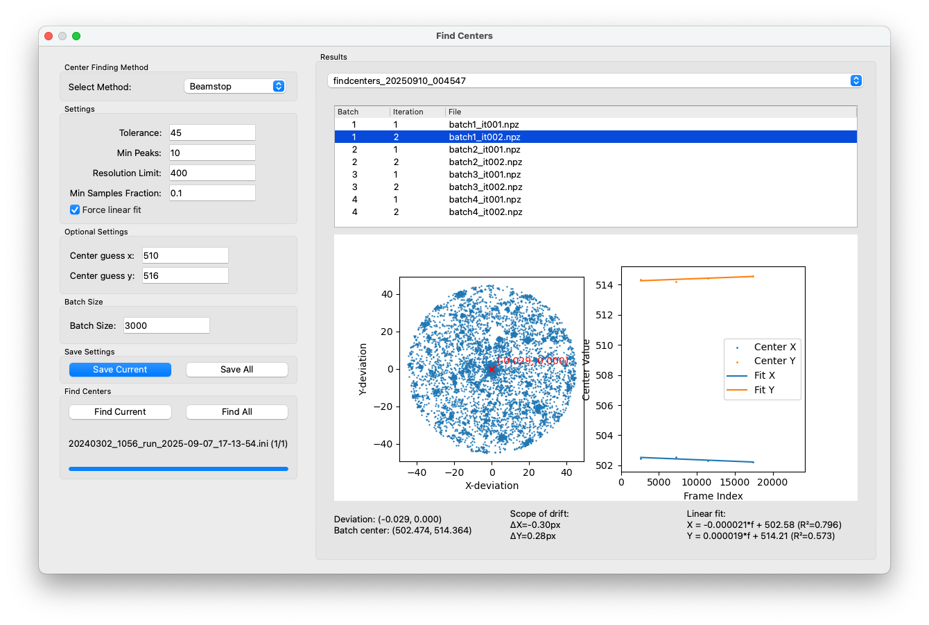
A good batch center is usually clearly visible in cluster plot (left). The right plot shows the linear fit.

Here are some good starting points for this dataset:

• tolerance: 10 px (You need to make an initial guess of the center position. Choosing a smaller value will speed up the process a little, but be sure to include the center.)

• min peaks: 10 (This is the minimum number of peaks a frame need to have to even be considered.)

• resolution limit: 500 px (Since most frames will have spots rather close to the center anyway (=low resolution), you can speed up center finding by limiting the cutoff to this range.)

• min samples fraction: 0.1 (This is a statistical parameter specifying the minimal fraction of centers to be part of a cluster, in order for the cluster to be accepted.)

• x0 and y0: 512, 512 (This are the coordinates of your initial guess. Since we aligned the beam close to the center of the detector, we use the center of our 1024 (binned) detector.

Refine Centers

Once we have a good idea of the general trend, we can attempt to refine the centers on a frame-by-frame basis. We do this by Locally Weighted Scatterplot Smoothing (LOWESS), where we try to fit many small linear models to subsets of data, and then form a distance weighted combination of them. This helps to smoothen out frame-to-frame noise.

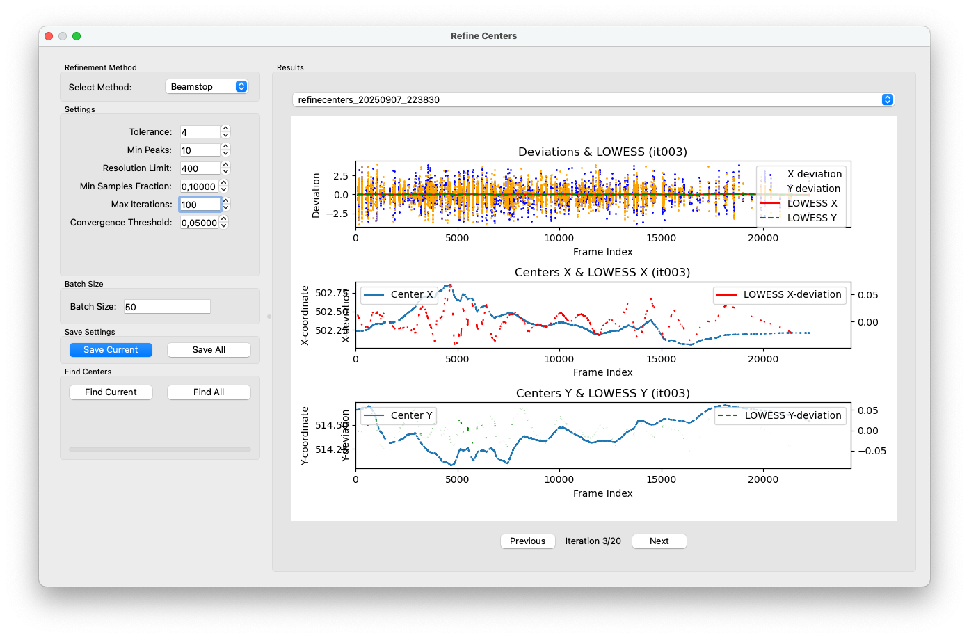
After a couple of cycles, you should see the LOWESS deviations to become smaller and smaller. The refinement loop breaks when the residual deviations are below the convergence threshold, or the maximum number of iterations is reached.

Note: The batch size is purely for computational performance tuning. You can usually ignore this setting.

Indexing & Integration

Once beam centers are refined, we are ready for try indexing. We are using a gradient decent algorithm called XGANDALF, which is part of the CrystFEL suite. This is where our dataset starts to turn into real crystallographic information. The program attempts to assign Miller indices to the observed reflections and extract their integrated intensities.

Open the Index & Integrate window from the workflow. On the left side, you will see a tree with all dataset files and their associated runs. Runs are self-contained folders created for each processing attempt, which makes it easy to try different settings without overwriting your earlier results. If you select multiple files that share the same run number, they will be processed together with synchronized settings.

The Settings tab on the right lets you configure the indexing parameters. You will notice that cell and geometry information are pre-filled either from the workspace or from earlier runs. Adjust tolerances, resolution limits, and integration radii to match your data quality. If you are unsure about the exact unit cell of your sample, start with more relaxed parameters and tighten them step by step.

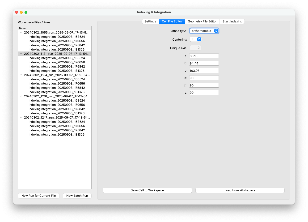
In the Cell File Editor, you define your targeted unit cell.

The geometry file is usually generated automatically based on your metadata. Still you should always check before running. If your dataset doesn’t index at all, oftentimes the detector coordinates are wrongly configured or the camera length is off.

When everything looks good, you can either run indexing for the currently selected file or start a batch run across the whole workspace. Batch runs will go through all files sequentially and show you which file is currently being processed. The output of each run is written to a .stream file. Keep an eye on the indexing rate.

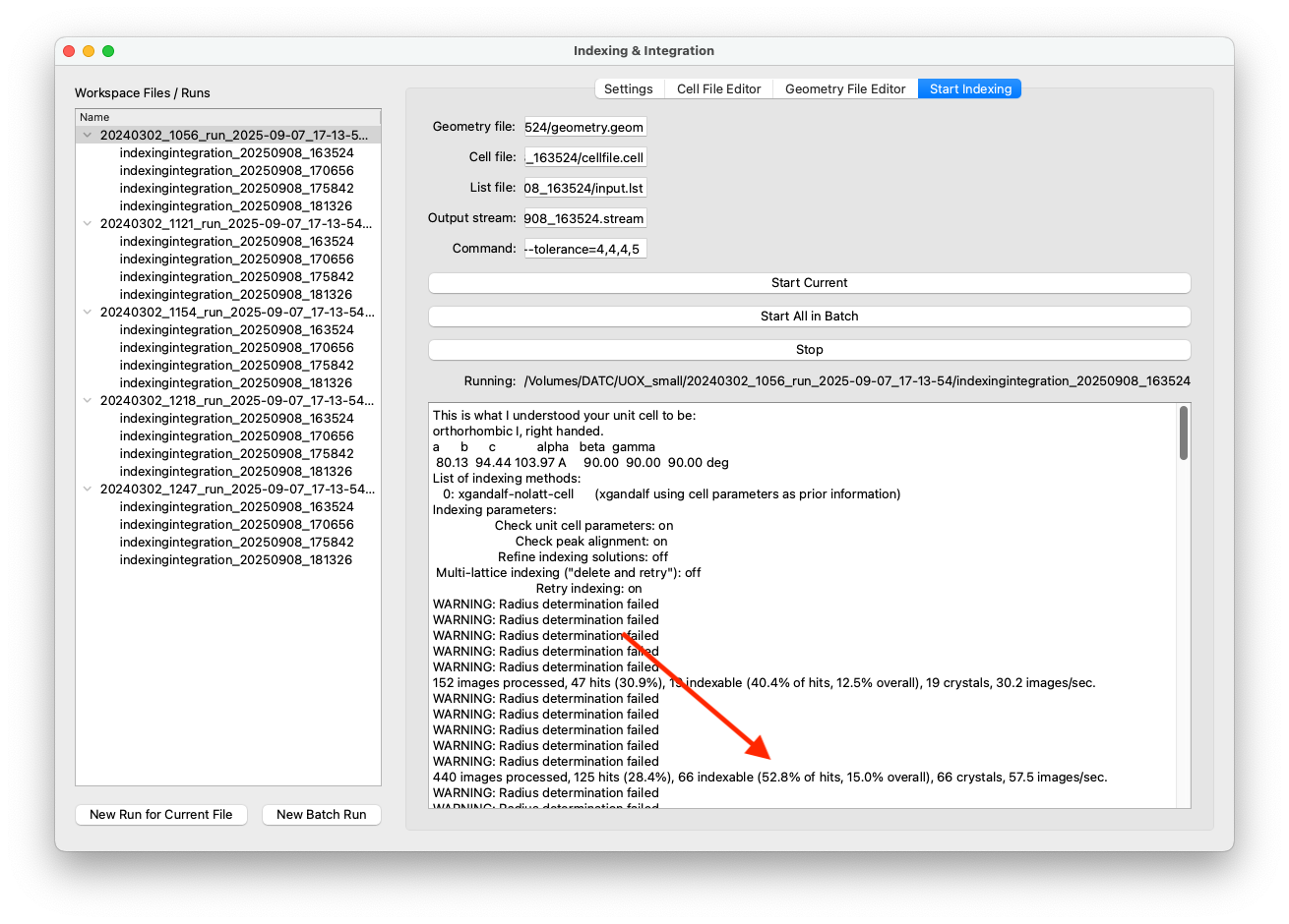
For the UOX dataset, you can take the following parameters as a reasonable staring point:

• tolerance: 4,4,4,5

• sampling pitch: 5

• gradient descent iterations: 2

FYI, this is the unit cell of UOX:

lattice_type = orthorhombic
centering = I
a = 80.13 A
b = 94.44 A
c = 103.97 A
alpha = 90 deg
beta = 90 deg
gamma = 90 deg

Note: Always check if your indexing results are sensible. Unfortunately this is not currently implemented in COSEDA - but will be soon. For now, you can open your stream file in CrystFEL to visualise your indexing results.

Merging

After indexing and integration, we combine our slices of data into a single, consistent reconstruction of reciprocal space. This step is performed with CrystFEL’s Partialator module, which scales and merges the intensities from all indexed patterns.

Open the Merge window from the workflow. In the first tab, you will see a list of available indexing runs across all files in your workspace. Runs with the same number correspond to the same processing conditions and are allowed to be merged together. When you select a run, the interface shows you how many files belong to it and lists all the associated stream files.

Click Generate Combined Stream to collect all stream files from the selected run into a single combined stream. A new folder will be created next to your workspace, named workspace_merge_. The combined stream file inside this folder will then serve as the input for Partialator.

In the Settings tab, you can configure the merging parameters. These settings control how intensities are scaled and combined across datasets. Once ready, press Start Merging to launch the process. Output and progress are continuously written to the log panel and statistics tab.

If you want to try different merging parameters, just restart the run: the software will create a new merge folder with a fresh copy of the stream file and your updated settings. This ensures you never overwrite previous results and keeps your processing reproducible.

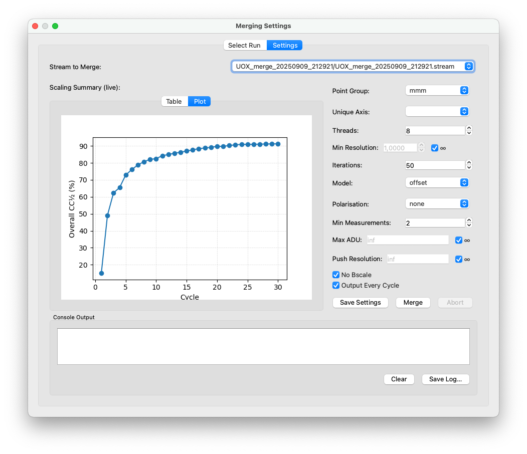
CC½ (or half set correlation) is the most important metric here. It is the correlation coefficient between two random halves of your dataset. It measures how consistently the same reflections are observed across different subsets, and should ideally converge towards 100%. Typically you can observer a saturation behaviour, as shown in the screenshot.

Some starting parameters:

• point group: mmm

• unique axis: leave empty

• threads: depends on your hardware, leave some headspace for other processes

• min resolution: 3

• iterations: 50

• model: offset

• polarisation: none

• min measurements: 2

• max ADU: inf

• push resolution: inf

• no bscale: check

• output every cycle: check

For each cycle, you will get an .hkl file, which you can use straight away for your structure solution.

Export

If you need an .mtz file, e.g., if you want to solve your structure using Phenix, you can use the export function to generate one.

Good luck!