MIL-101(Cr) Tutorial

Download Tutorial Dataset

You can download a tutorial dataset of MIL-101 here.

Open Dataset

To save some time for the import, I already converted the datasets from Velox/.emd format to HDF5. Once you unzip the fild, you should see the following folderstructure:

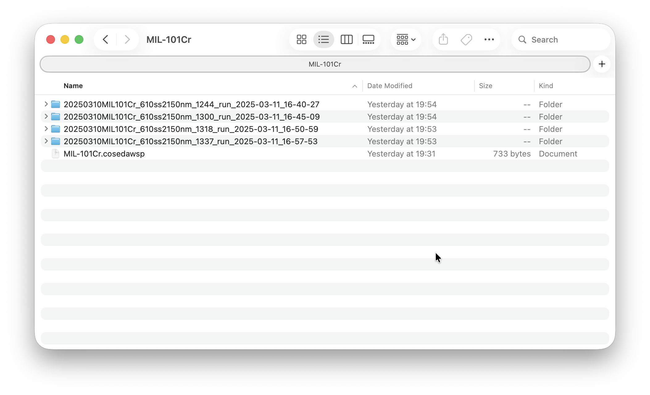
There is a workspace file (.cosedawsp), and a subfolder for each dataset. The idea of a workspace is to enable batch processing of a dataset which is split over serveral files. The workspace file references the datasets, stores project wide information like a unit cell, and a few UI settings. Workspace files allow you to quickly switch between projects - all settings are autmatically restored. Each dataset folder contains an .h5 file, an .ini file and a .log file, as well as some subfolders with processing artefacts.

For processing your own project, simply create and save a new workspace, and use one of the import tools (File > Import) to add you datafiles.

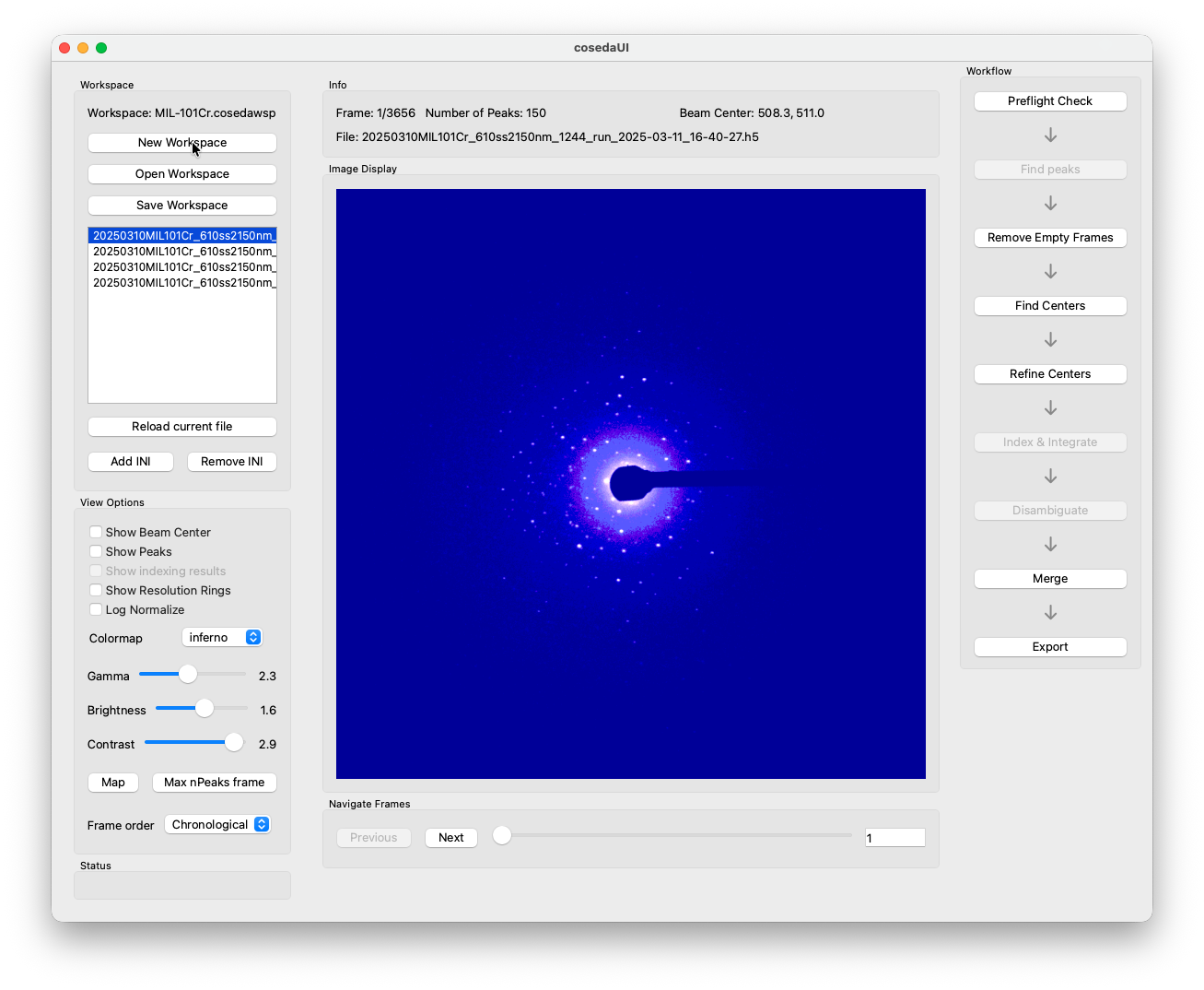
View Options

Use the controls in the View Options box to adjust the preview to your needs. You might notice that in the beginning, some of the toggles are greyed out. They will become active once the required data is present in the file. View opions will be saved in the workspace file and should be recovered autmatically upon opening a file.

Workflow

The left panel shows the workflow for processing c-SerialED data. You can click through the process step by step.

Tooltips

As of May 2026, most input fields have tooltips. If you are unsure settings to choose, hover with the mouse pointer over the input field. After a short moment, a hint should pop up. If you discover any missing information, please report it here contact-project+kristallorakel-coseda-reportissue@incoming.gitlab.com

Preflight Check

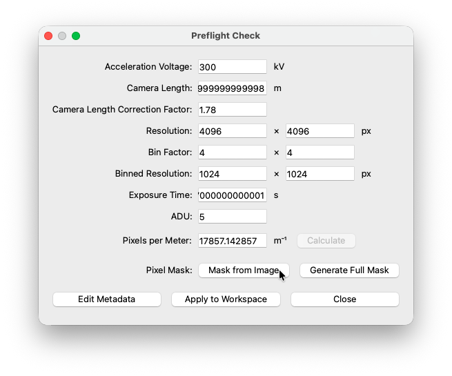
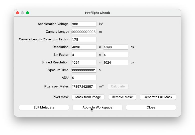
When using one of the importers, COSEDA will try to parse all necessry metadata from the original file. If for some reason, a piece of information can not be parsed, you can add it manually to the preflight check.

Acceleration voltage

Used to calculate the electron wavelength.

Camera length

Detector distance/camera lenght in meters as reported by the microscope. This is in most cases parsed autmatically.

Camera length correction factor

Unfortunately it is very common that the camera length reported by the microscope is not correctl. Often it can be corrected by a constant factor. Get this factor by asking your facility staff or calibrate yourself using a standard sample.

Resolution

This should be the full resolution (unbinned) of your detector. This and the bin factor are important to calculate the correct physical pixels size.

Bin factor

Used to calculate the actual resolution of the data.

Binned resolution

Autmatically calculated from detector resolution and bin factor.

Exposure time

Currently not relevant for processing pipeline - but reported for good measure ;-)

ADU

Analog-to-Digital Unit: This is a detector specific constant describing the relationship between the raw signal and the digital value stored in the file. Consult detector data sheet or facility staff if you are unsure.

Pixels per meter

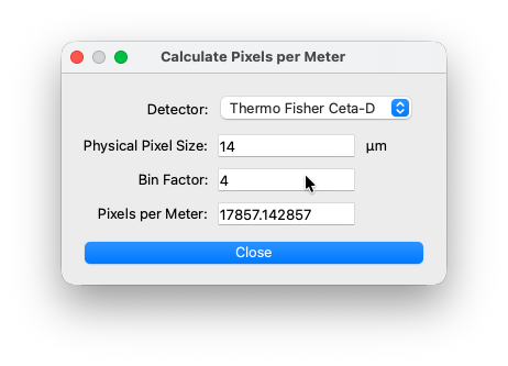
Reciprocal of the physical spacing of the dector pixels. You can use the calculator tool or manually add a value. In the calculator, select one of the hardcoded presets or add the physical pixel size manually (see datasheet of your detector). The calculated result is automatically transfered to the main window.

Mask

If you do not want to mask out anything, click the Generate Full Mask button. If you used a beamstop, you can draw a black (invalid pixels) and white (valid pixels) image in your graphic program of choice and import it through the Mask from Image button.

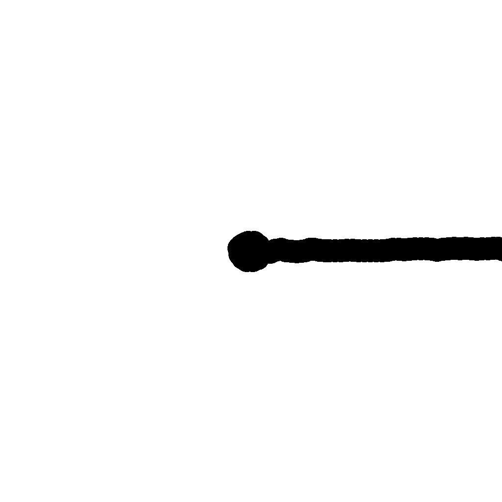
Note: The tutorial data already contains a valid mask. You can skip this step!

Apply to Workspace

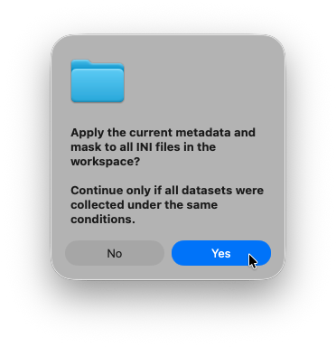
Once you made sure all settings are correct, press the apply to workspace button. The settings you made will be applied to all datasets in the workspace.

You will be prompted to confirm the changes.

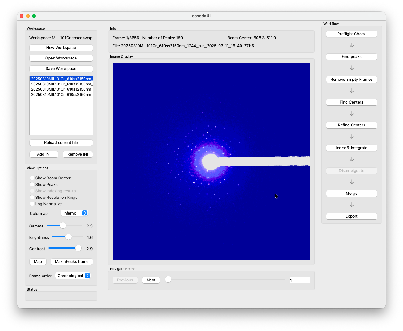
If you added a mask, you should now see the mask applied to the preview. If not, reload the file.

Peakfinding

Currently 2 peakfinding alogrithms are implemented. peakfinder8 from Robert Buecker’s diffractem package, as well as a homebrewed implementation of peakfinder9.

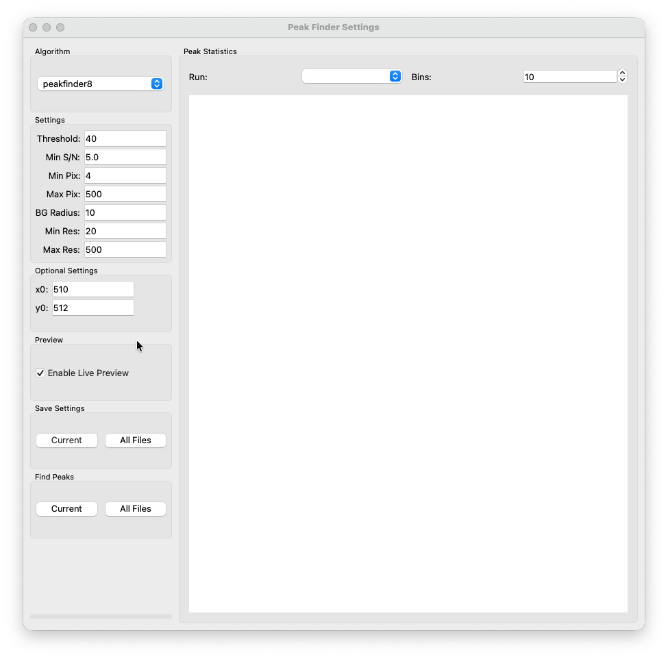
Upon ticking the Enable Live Preview box you should see peak markers appear in the preview image in the main window. Use them to tune the parameters for your specific dataset. Once you found good defaults for your detector there is usually not much tewaking required.

Threshold

This is the minimum intensity a candiate pixel needs to have to be considered. If you have no idea where to start use the ![Inspect Image] tool. Draw the box over a weak peak far away from the direct beam. A popup with the magnified cutout will appear. Read the values of the brightes pixels. Start with a value slighly below that. If you see a lot of noise being picked up, increase the value. If you see even weaker peaks not being picked up, decrease the value.

Min S/N

Minimum signa-to-noise ratio of a candiate peak to be considered. This depends a lot on the type of detector (CMOS/Hybrid Pixel). If you have no idea, start from e.g., and try to reduce/increase in samll increments. Observe the change in the preview - same principles as for the threshold.

Min Pix

Minimum size of a candiate peak to be considered (in pixels). It prevents hot pixels from being identified as a peak. This depends mostly on the physical pixels size of your detector. Once you found your default ususally no tweaking is required.

Max Pix

Maximum pixel size. Prevents large bright regions being identified as a single peak. Usually no tweaking required.

BG Radius

This is the local background radius of a peak used to detemine the peak intensity.

Min Res

Minimum resultion - minimum distance a candidate peak needs to be away from the direct beam (in detector pixels) to be considered. This setting is meant to prevent bright pixels in the halo of the direct beam to be mistaken for a peak.

Max Res

Maximum resoution. Usually set to cover the entire detector.

x0/y0

Give the peakfinder a rough estimation of the direct beam position. This does not need to be very accurate but is required for min/max res filtering. You can set it by clicking in the input field: The cursor will turn into a crosshair. Click the estimated center position in the preview in the main window. The coordinates will be automatically transferred.

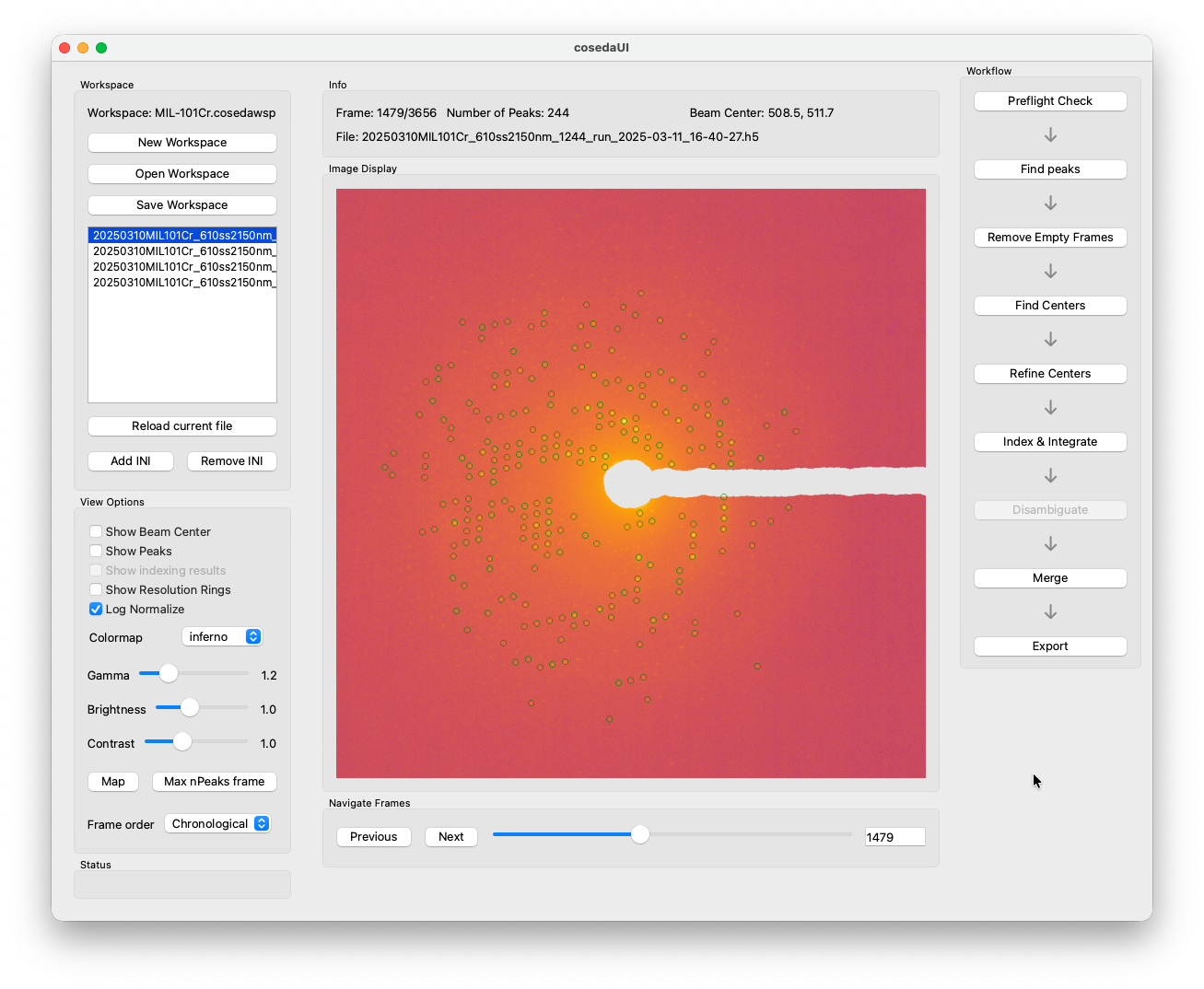
You can use the Navigate Frames controls to shuffel around between frames to check the settings. You can also use the filetable in the Workspace controls to switch between files at any time. Once you are happy with the live preview, save them and click Find Peaks → All Files to run on all datasets in the workspace.

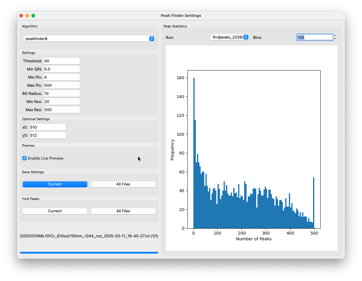
After a short while (dependent on the size of the dataset and your hardware) a histogram will show up in the right section of the peakfinding window. It shows the distribution of the number of peaks found per frame for the current run. A typical result looks like a broad distribution skewed towards low counts — most frames will have relatively few peaks, with a long tail of brighter frames. The exact shape will depend a lot on your sample.

A side note on data provenance

Once peakfinding (or any other processing step) has started, you should see a new timestamped run folder appear in each dataset folder.

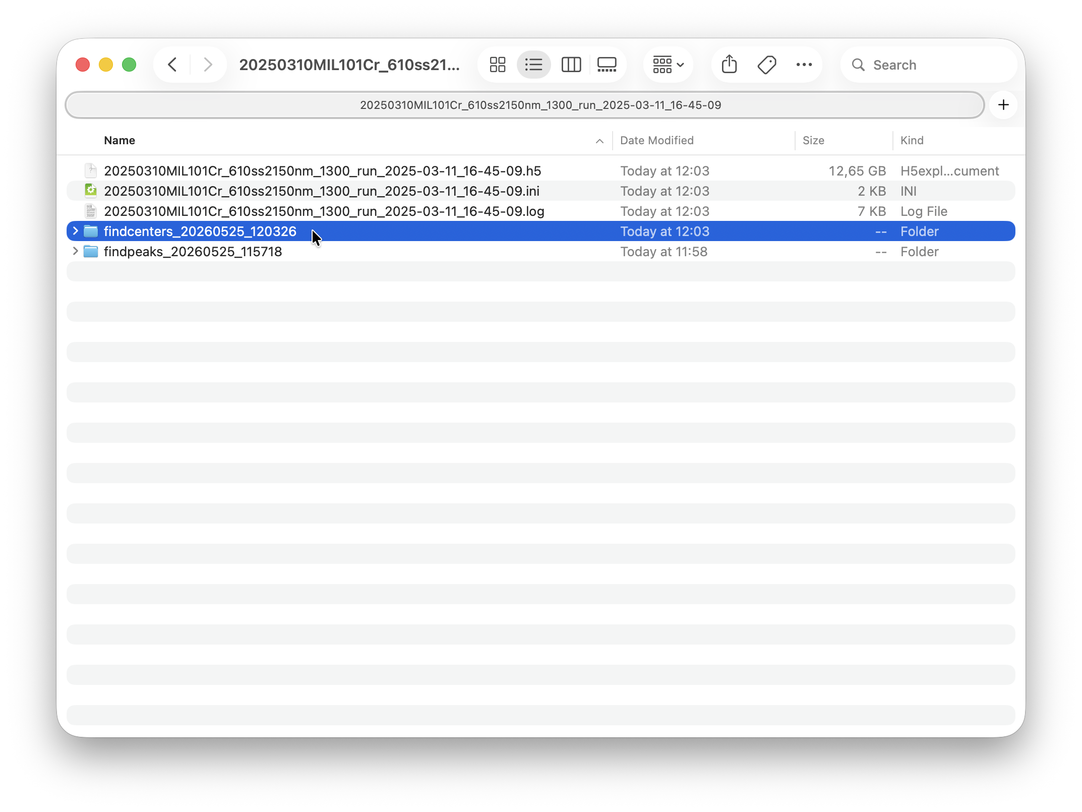
Each run folder contains the peakfinding outputs and a few diagnostic plots. These will never be overwritten. Often you may want try a processing step several times with different settings. While processing outputs in the HDF5 file are updated, the artefacts in the runfolder will never be overwritten. You can come back at any time to compare output from previous results. Each runfolder also contains a parameterdump file, which is just a text file logging the settings used in each run.

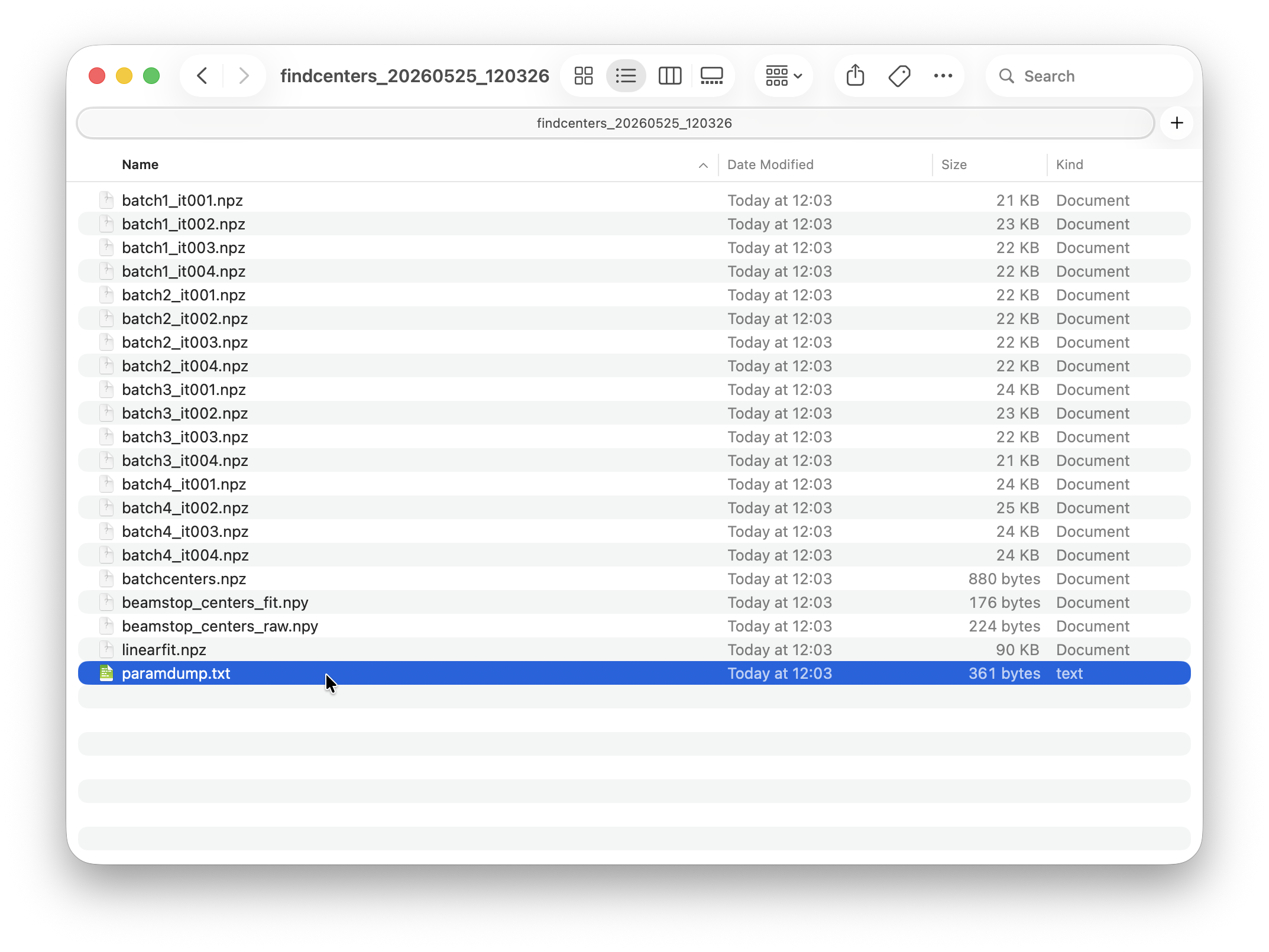
All processing steps from peakfinding to indexing happen on a dataset level. Their outputs folders will therefore end up in the respective dataset folder.

Everything after happens on a workspace level. The run folders for the processing steps will therefore appear aside the workspace folder.

Remove Empty Frames

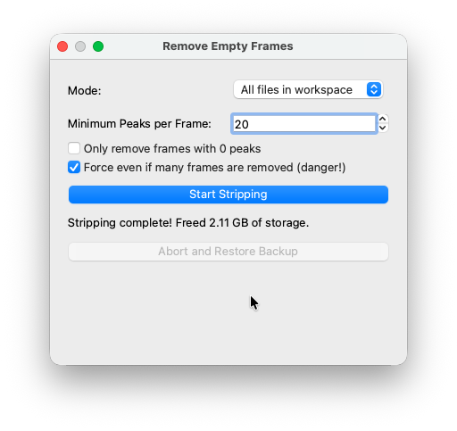
A typical c-SerialED dataset contains a large number of frames where no crystal was in the beam. These frames do not contribute anything useful but take up disk space and slow down all downstream steps. The Remove Empty Frames step strips them from the HDF5 files in-place.

Indexamajig, the currenly used indexing engine struggles with frame containing less then 20-25 reflections. To save time and space, we can therefore optionally set a stripping threshold (Minimum Peaks per Frame) larger than 0, e.g., 20.

Filestripping is irreversible! If the run will remove a large portion of the dataset, the software will demand you to acknowledge this. Make youre your peakfinding settings were reasonable before you continue.

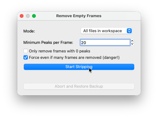
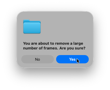
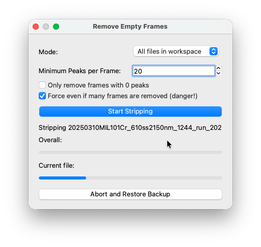
Once complete, COSEDA reports how much storage was freed. For this 10GB dataset, stripping freed over 2 GB.

To save time and space, this was already done in the tutorial dataset - so do not expect large wins in this step here.

Find Centers

It turns out that most indexing algorithms like indexamajig, the one we use in COSIDA are highly sensitive to an accurate prior knowledge of the beam center. We do this in a two step process. Open Find Centers window from the workflow panel. Since this dataset was collected on a Ceta-D with a beamstop, select Beamstop as the method. There is another direct method implemented, however this one is still in an experimental state. The Beamstop method works reliably on both datasets with and without beamstop.

Tolerance

This specifies the search radius around our intial center guess in pixels. As long as the true center is withing the search radius around the guess, this should not change the outcome. A larger tolerance may increase the compute time.

Min Peaks

The algorithm works by identifying Friedel pairs (reflections related by inversion symmetry through the direct beam). For every peak at position p relative to the beam center, there should be a corresponding partner at −p. The code searches for peak pairs whose vector sum (relative to the current center guess) falls within the Tolerance radius. The midpoints of these pairs cluster around zero when the center is correct. Their offset reveal the direction and magnitude of the error.

Frames with too few peaks are unlikely to yield enough valid pairs to contribute a useful signal, so Min Peaks sets a hard threshold. Frames with fewer reflections than this value are skipped entirely. From our experience a value auround 20 is a sensible starting point. Increase it if the deviation scatter looks noisy.

Resolution Limit

Only peaks within this distance from the current center estimate (in detector pixels) are considered for Friedel-pair matching. Low-resolution reflections close to the direct beam tend to be reliable enough, so restricting the search to a limited radius (e.g. 200 px) keeps the computation fast while concentrating on the strongest signal. Increase this value if your crystal produces sparse diffraction or if useful peaks are located further from the direct beam.

Min Samples Fraction

After accumulating the Friedel-pair midpoint deviations for an entire batch, the algorithm clusters them with DBSCAN and fits a Gaussian to the largest cluster. This parameter sets the minimum fraction of all collected deviations that must belong to a single DBSCAN cluster for it to be accepted as valid. A lower value allows sparser clusters through. A higher value demands a tighter, more confident result. The default of 0.1 works well for most datasets.

DBSCAN eps

The neighborhood radius (in pixels) that DBSCAN uses when clustering the deviation cloud. Two deviations are considered neighbors if they lie closer than this value. The default of 5.0 works for most datasets. Lower it if your deviations are very tightly clustered, or raise it slightly if the algorithm fails to find a cluster on a dataset you expect to be clean.

Center guess x0 / y0

An initial estimate of the direct beam position in detector pixels. The algorithm will converge to the true center as long as this guess falls within the Tolerance radius of it. You can populate these fields the same way as in peakfinding: click the input field to activate coordinate picking, then click the estimated beam position in the main window viewer. If left empty, COSEDA defaults to the geometric center of the frame.

Batch Size

Typically during the collection of a c-serialED dataset, we do not deliberalety move the beam. However a slow drift of the beam center can often be observed. To account for this drift, frames are divided into batches, and one center estimate is derived per batch. These batch centers are then combined into a drift model. Smaller batches provide finer sampling of beam drift but require more peaks per batch to yield a clean deviation cluster. A few thousand frames per batch is usually a reliable starting point. You can set whatever number you like, however, the algoirthm will make sure that there are at least 4 batches per dataset and autmatically overrides the batch size if necessary. If the deviation scatter plot shows no clear cluster, try increasing the batch size to accumulate more Friedel pairs. If processing runs out of memory, reduce it. (see note on parallelism)

Once you are happy with the settings, save them with Save Current or Save All, then click Find Centers → Current or Find Centers → All to run on the dataset(s).

After a short while, batch results should show up in the table on the right side. If you click on one of the batches, the results panel will show a scatter plot of the per-frame center deviations relative to the batch center on the left side. A tight, clearly visible cluster around zero in the deviation plot indicates a good result. Once all batches are done, a linear fit of the center drift over frame index will appear on the right. A (more or less) linear behavior is what we expect, so in this case the fit looks reasonable.

You might have noticed that there are some additional tickboxes to enforce a linear fit (even if the batch results do not behave linear), and a setting to skip the fit and continue with batch data. These are addional tools to tinker in special cases (e.g., very large continuous datasets and unstable beam), but are generally not recommended.

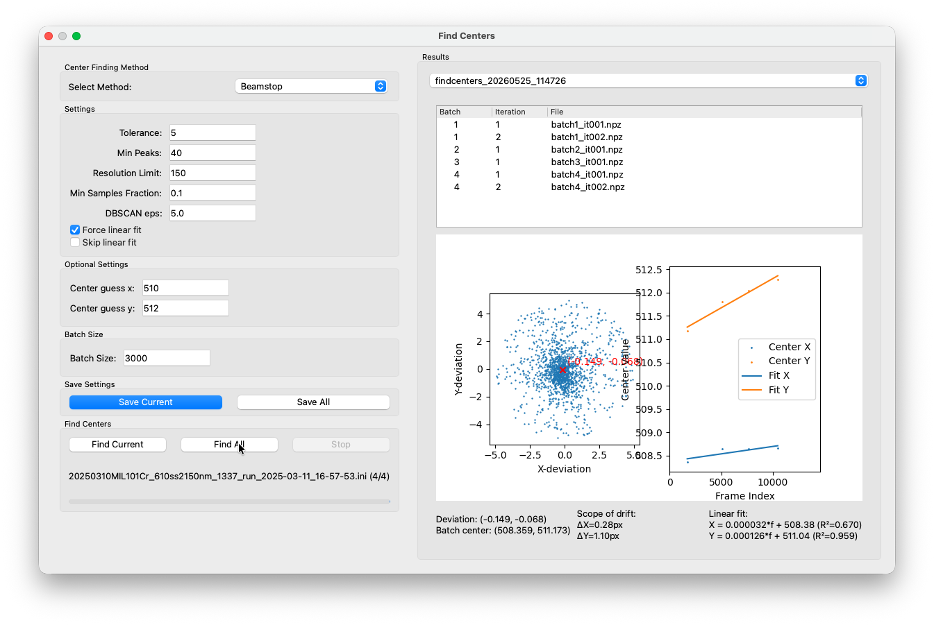
After the fit, the algoirthm will interpolate frame-by-frame centers (under consideration of time series gap from stripped frames) based on the fit and write the updated centers are back to the HDF5 file. As mentioned above, plots etc. are written in their own run folder and stored permanently. Feel free to do several runs and play with the paramters to get a feeling for how it works.

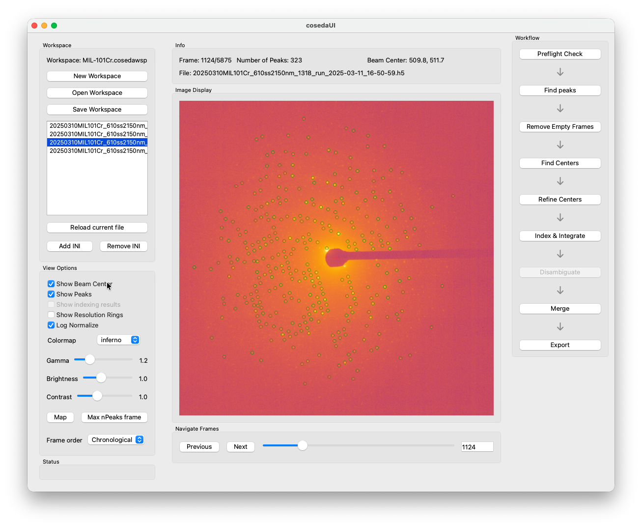
Back in the main window, the tickbox for the beam center overlay in the preview should now be ungreyed.

A side note on parallelism

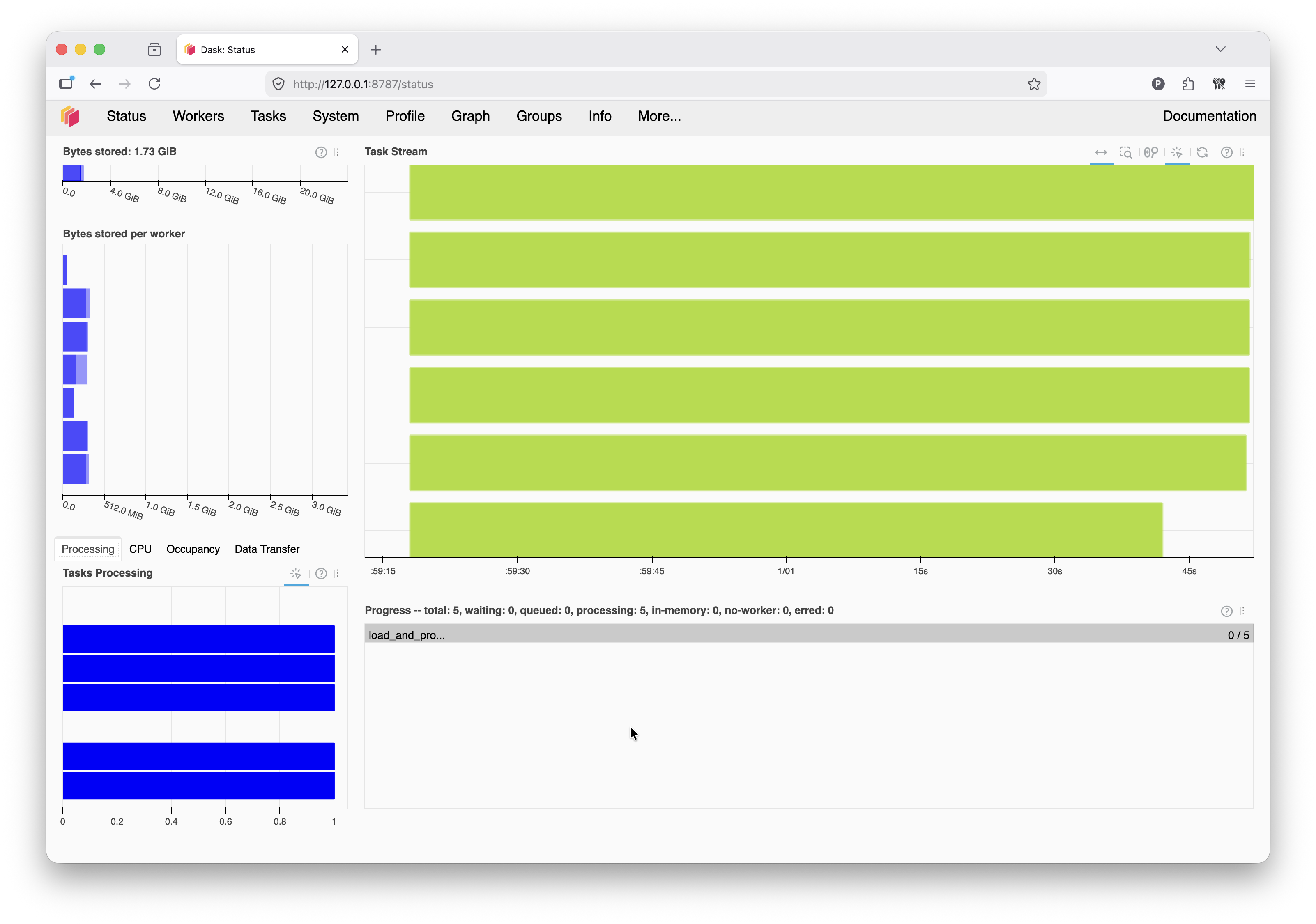
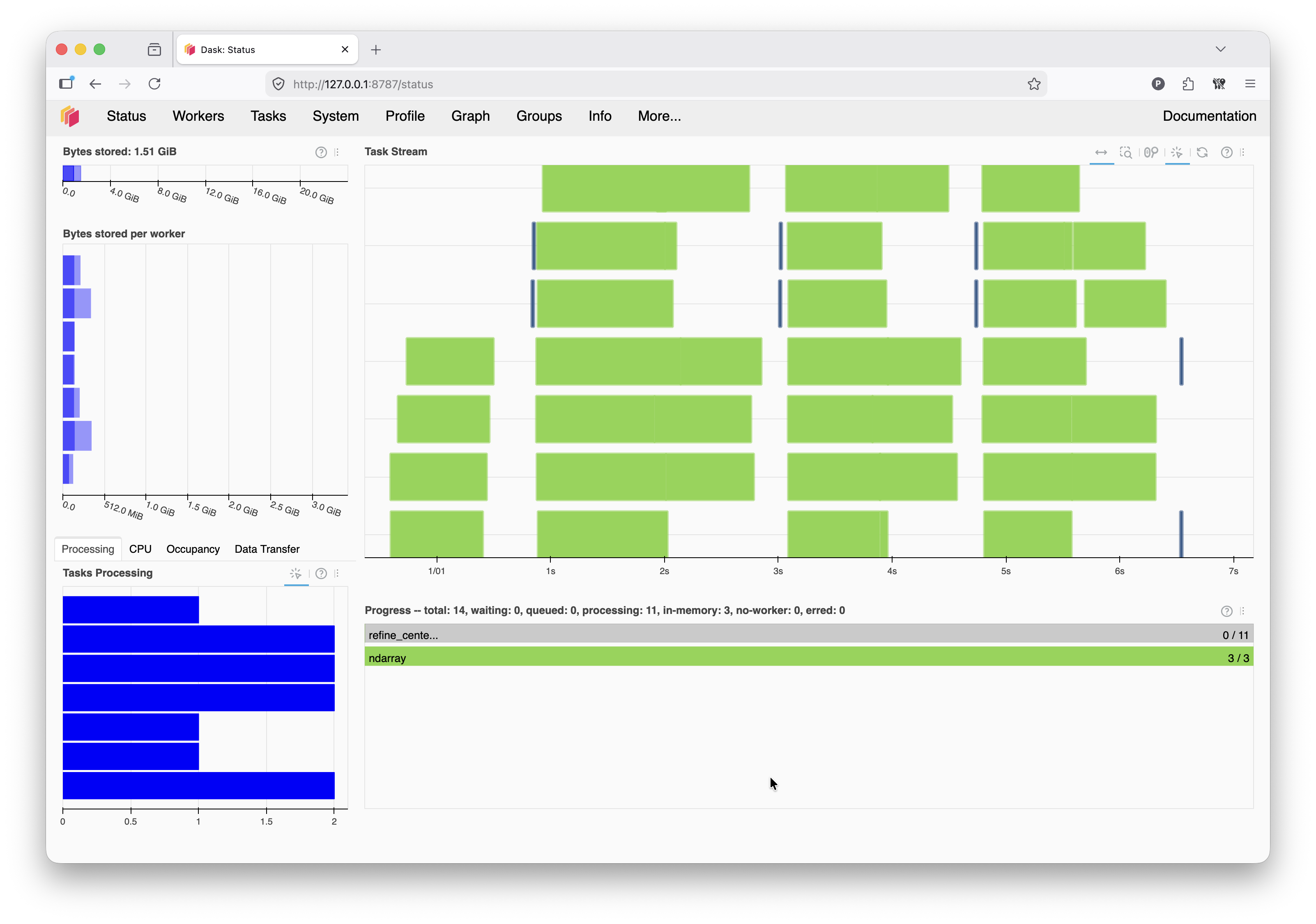
COSEDA uses Dask for parallel processing. From the menu bar, you can open the Dask dashboard. This is generally not needed but can be helpful for debugging in case processing crashes.

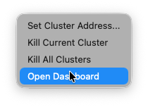
From our experience, most crashes are caused by memory overflows. You can see the memory consumption per worker in the dashboard. If one or more workers get dangerously close to the limit, try reducing the batch size.

Refine Centers

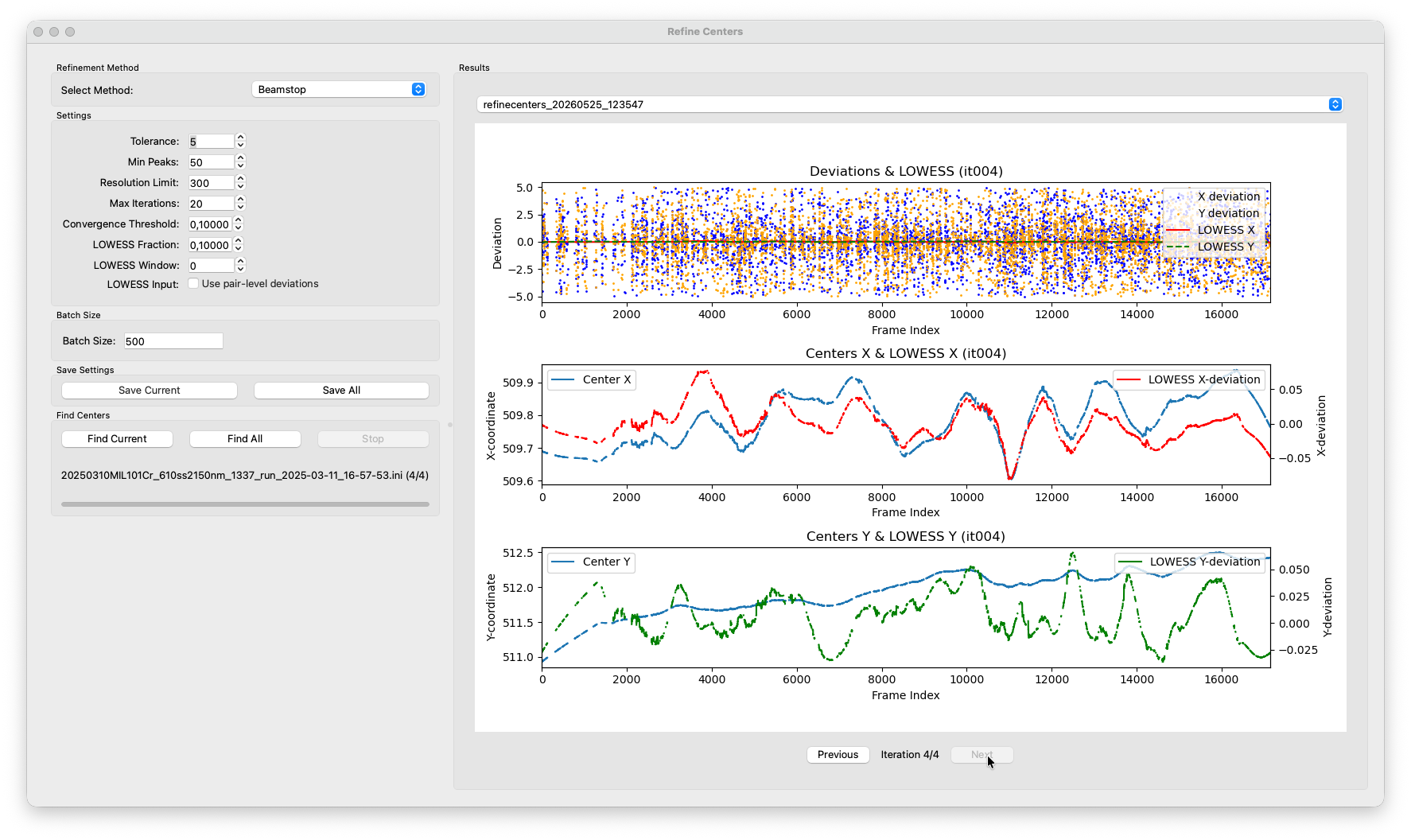
Find Centers already interpolates a per-frame center for every frame, but that interpolation is based on a linear drift model fitted through the batch estimates. Any non-linear component, like a slow curve, a sudden jump or jitter is not captured. Refine Centers corrects for this. It re-runs the Friedel-pair deviation measurement individually for every frame, using the current per-frame center as the starting point, and smooths the resulting deviations with a LOWESS (Locally Weighted Scatterplot Smoothing) fit. The centers are then nudged by half the smoothed correction, and the whole process repeats until the corrections become negligibly small.

LOWESS is non-parametric. It fits the data locally using a sliding window. That means it will naturally follow the actual drift curve without you having to choose a model.

Open Refine Centers from the workflow panel. As before, select Beamstop as the method.

Tolerance

Same meaning as in Find Centers: the Friedel-pair search radius in pixels around the current per-frame center estimate.

Min Peaks

Same as in Find Centers: frames with fewer reflections than this value are skipped.

Resolution Limit

Same as in Find Centers: only peaks within this distance from the current center estimate (in detector pixels) are used.

Max Iterations

A hard cap on the number of refinement passes. The algorithm stops early once convergence is reached, in practice it often won’t hit this limit. Usually covergence is reached within a few cycles. You can set it to 10 or 20. If you hit the limit without convergence, this should be interpreted as warning sign. Go back and check if your settings are reasonable. From experience, in most cases the Convergence Threshold is set unrealistically low. If you play around too much, sometimes you might navigate into a dead end or oscillation behavior. In this case, just rerun your latest centerfinding to “reset”.

Convergence Threshold

The refinement is considered converged when the LOWESS-smoothed deviation is below this value (in pixels) for every frame in both X and Y simultaneously. The default is 0.1 px. If the algorithm never converges on an otherwise clean dataset, try relaxing this slightly.

LOWESS Fraction / LOWESS Window

These control the smoothing bandwidth. In other words, how many neighboring frames contribute to the local fit at each point. LOWESS Fraction expresses this as a fraction of the total frame count. LOWESS Window sets it as an absolute number of frames and overrides the fraction when greater than zero. A fraction of 0.1 is a safe default for most datasets. For a rapidly changing drift you may want a smaller window to avoid over-smoothing. For very noisy datasets a larger window gives a more stable result. If you have huge datasets (e.g.; 100k frames in a single file), setting a window manually rather than setting a fraction may be preferrable. The fraction and absolute window size are mutually exclusive and the absolute window will override the fraction.

Batch Size

Same role as in Find Centers: frames are chunked for Dask parallelism. 500 frames per batch is the default and works well in most cases. Reduce it if you run into memory issues. Unlike for the center finding, here the batch size setting is purely for compute speed optimization and will have no effect on the outcome.

Once you are happy with the settings, save them and click Refine Centers → Current or Refine Centers → All.

With each completed iteration, a new entry appears in the results panel. The plot shows the per-frame Friedel-pair deviations as a scatter, with the LOWESS fit overlaid. You should see the scatter tighten and the LOWESS line flatten toward zero with each pass. That is the refinement converging.

Keep in mind that axis limits are scaled to fit the deviations in each iteration. Just because the deviations still span the entire plot range, does not mean that the iterations did not make any progress. This has caused confusions before.

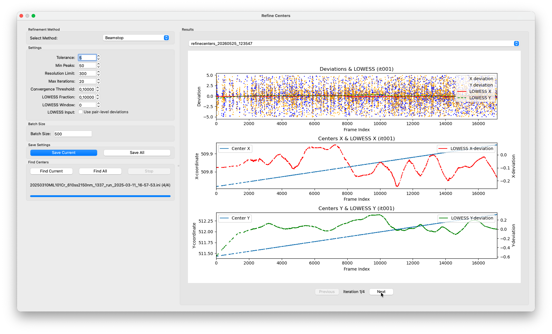
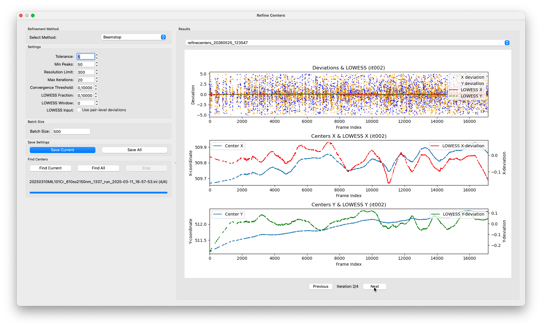
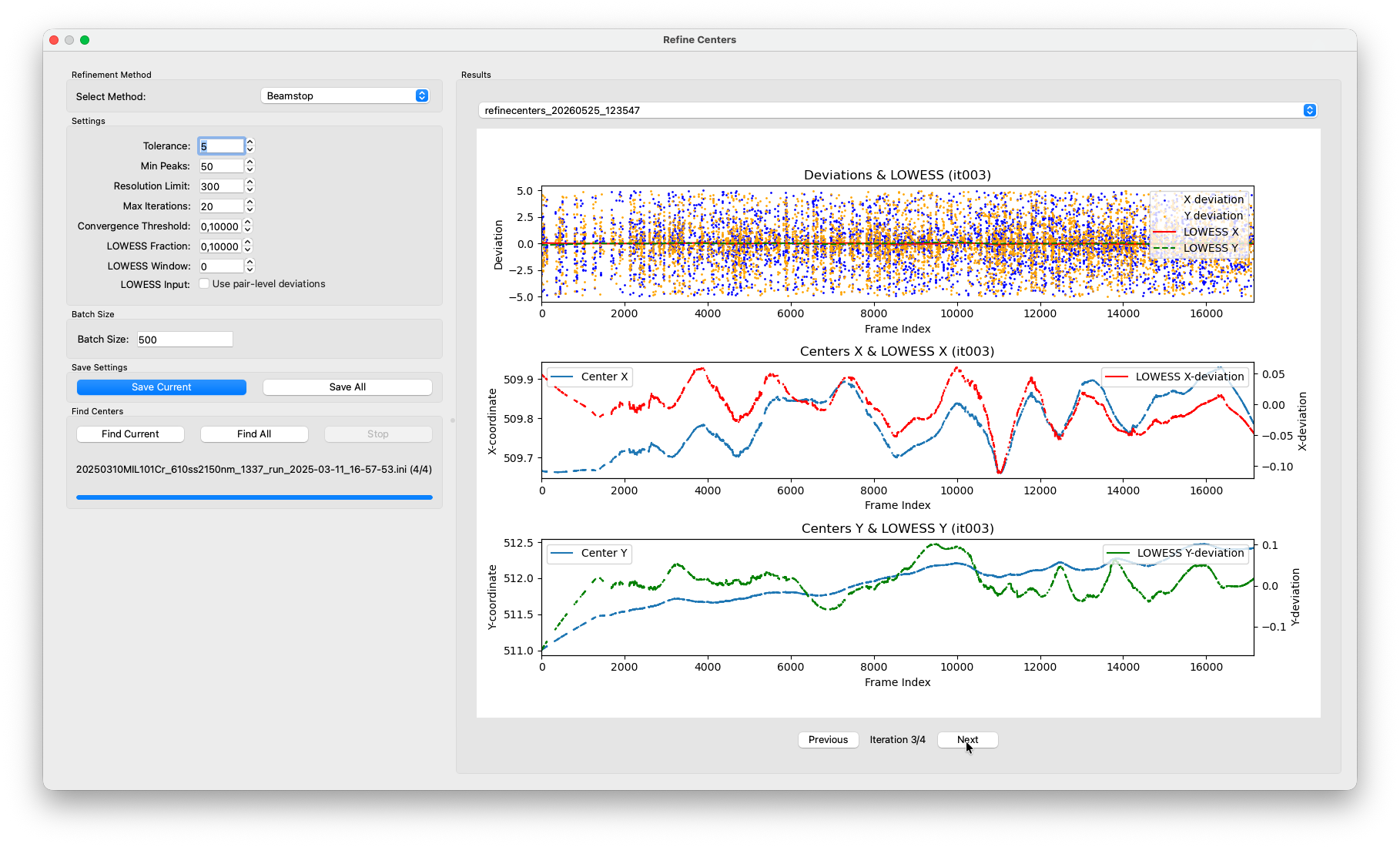
After a few iterations the residual deviations should be well below 1 pixel. Once converged, the algorithm stops automatically and writes the final per-frame centers back to the HDF5 file.

Again, you can watch the Dask dashboard if you want to monitor progress.

Index & Integrate

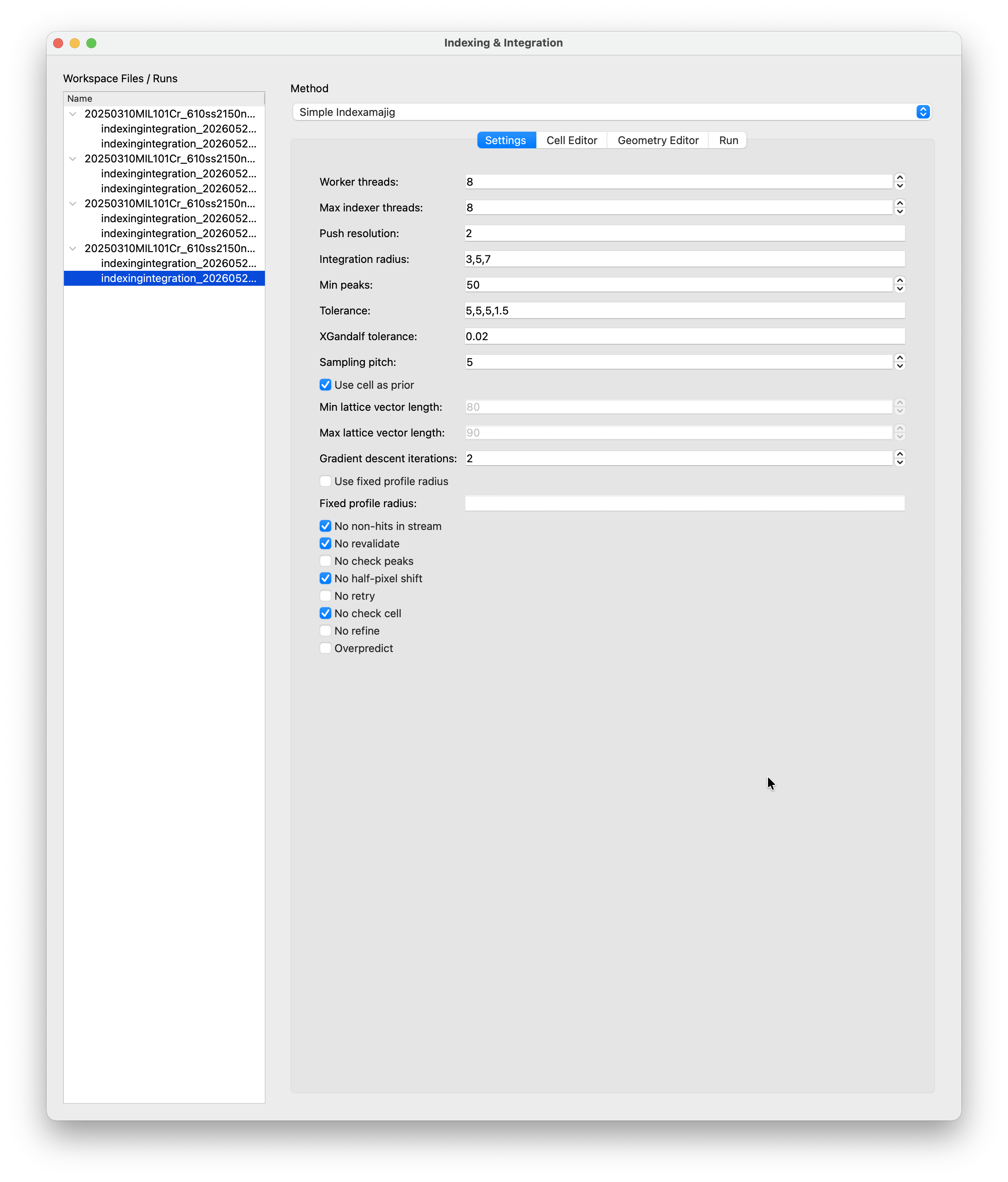
Open Index & Integrate from the workflow panel and select Simple Indexamajig as the method. Indexamajig is the CrystFEL program COSEDA calls for indexing and integration. In this workflow we use the XGandalf indexing algorithm. The indexing window has three tabs: Settings for the indexamajig parameters, Cell Editor to define the unit cell, and Geometry Editor for the CrystFEL geometry file. Fill in all three before running.

Worker Threads / Max Indexer Threads

Worker Threads sets the total number of indexamajig threads (-j). Max Indexer Threads sets how many of those are used per pattern. Set both to the number of CPU cores you want to dedicate to the job.

Push Resolution

Integrate peaks slightly beyond the apparent resolution of each pattern (in 1/nm). For this dataset we use 2. If you are unsure, start with a small value like 0.5 and increase it if you want to push to higher resolution.

Integration Radius

Three comma-separated pixel radii defining the inner, middle, and outer integration rings (--int-radius). The inner ring covers the peak, the region between inner and middle is the gap, and the region between middle and outer is the background annulus. These depend on the physical size of peaks on your detector and typically need some tuning. For this dataset 4,5,8 works well.

Min Peaks

Minimum number of peaks a pattern must have to be sent to the indexer. Patterns below this threshold are skipped entirely. Set this consistent with the stripping threshold used in Remove Empty Frames.

Tolerance

Tolerances for comparing the indexed cell against the reference cell, e.g. 5,5,5,1.5. The first three values are percentage tolerances for a, b, and c. The last value is the angular tolerance in degrees. Only relevant when No check cell is unticked.

XGandalf Tolerance

Relative tolerance on the indexed lattice vectors (default 0.02 = 2%). If your indexing rate is low, you might want to increase this intially. Though you should always check manually if your indexing results are sensible and match the observed peaks. You may then use the cell fit tool to propose a refinde cell as a proposal for a subsequent indexing run with tighter tolerances.

Sampling Pitch

Controls the density of the initial reciprocal-space sampling in XGandalf, on a scale of 0 (coarse) to 7 (fine). Higher values are more likely to find a solution but are slower. The default of 5 is a good balance.

Use Cell as Prior

When checked (default), the cell definition is passed to indexamajig and XGandalf uses it as a starting point for its gradient descent. This is the normal mode when the unit cell is (roughly) known. Uncheck for a free-lattice search. This is useful if you do not know the cell and want XGandalf to find it from scratch, in which case the min/max lattice vector length fields below become relevant.

Gradient Descent Iterations

Number of gradient-descent refinement steps XGandalf performs after finding an initial solution (0–5). More iterations improve accuracy at the cost of compute time. The default of 2 is sufficient for most datasets.

Flags

The checkboxes at the bottom expose common indexamajig flags. The defaults are appropriate for c-SerialED data from COSEDA and rarely need changing. The most relevant ones to be aware of:

• No check cell: skip comparing the indexed unit cell against the reference cell. This is enabled by default. The cell check can discard valid solutions that index slightly outside the tolerance, so it is usually left off.

• No refine: skip CrystFEL’s prediction refinement step after indexing. This is not the same as the COSEDA center refinement above. Prediction refinement tries to improve the indexed solution before the final predicted reflections are used. Skipping it makes the run a bit simpler and faster, but can reduce the quality of the result and may let false indexing solutions through. If the predicted spots look slightly off, try unticking this option.

• Overpredict: predict reflections beyond the observed peaks, increasing the number of integrated intensities.

Cell Editor

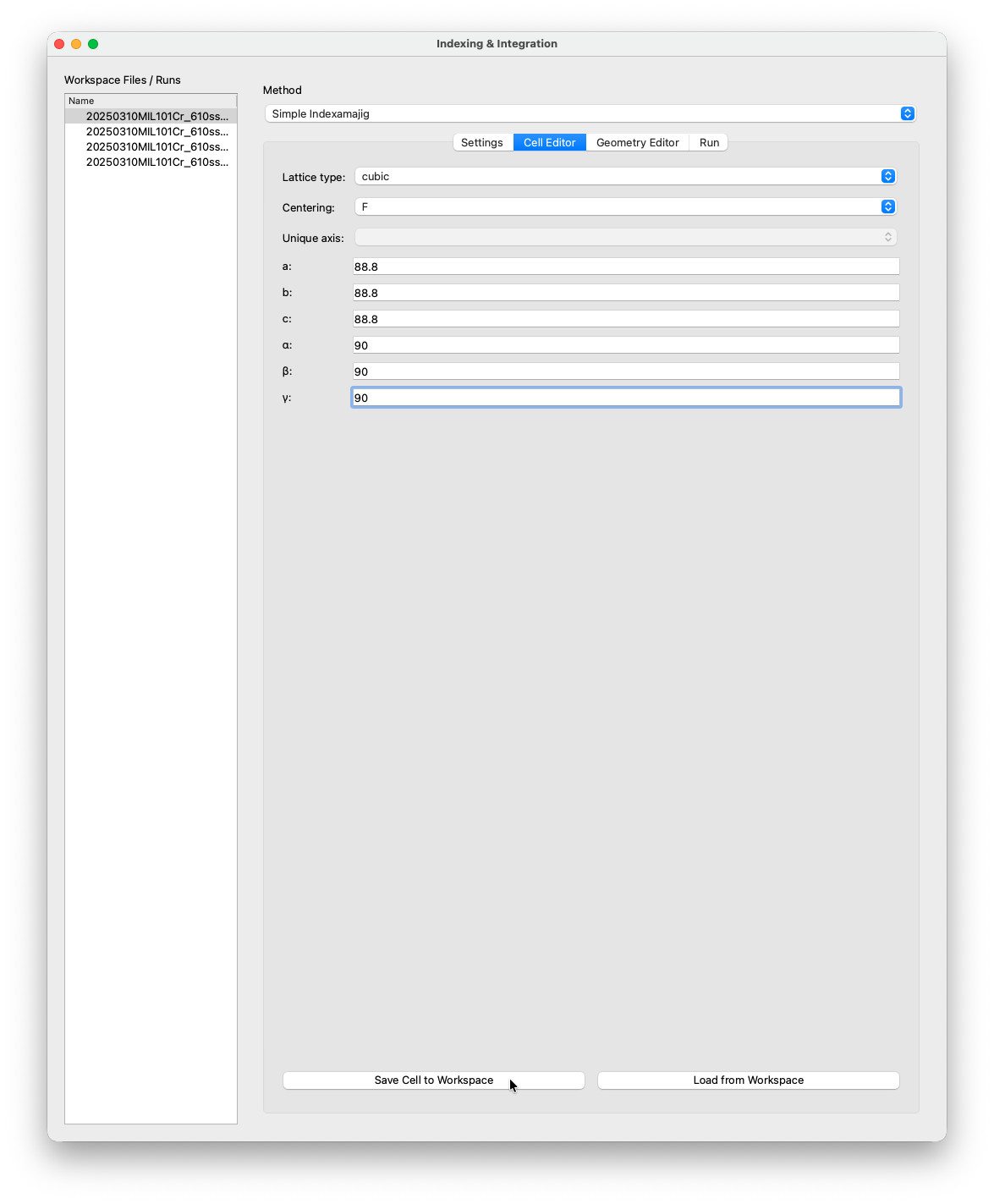
Enter the unit cell in the Cell Editor tab. For MIL-101(Cr) a reported cell in literature is cubic F with a = b = c = 88.8 Å.

Geometry Editor

The Geometry Editor tab lets you inspect and edit the CrystFEL geometry file. For single-chip detectors, clicking Generate Single-Chip Geometry is sufficient. COSEDA will generate the description autmatically from the metadata.

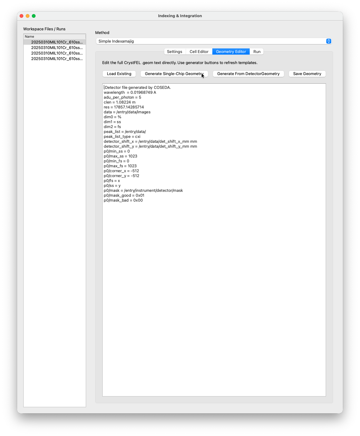
Once you are happy with the settings, switch to the Run tab and click Index & Integrate. You will see a new run appearing in the tree on the left. You can follow the output live in the console.

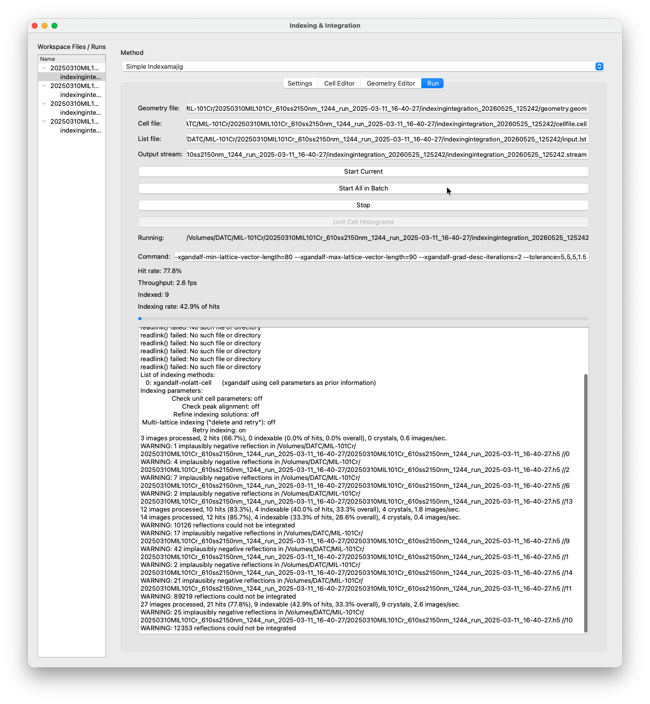
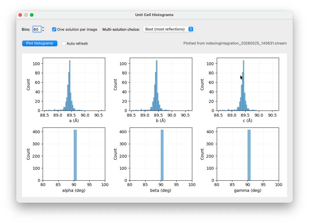
Additionally a unit cell histogram window with the already finished indexing solutions will pop up. The histogram is updated every 60 seconds by default.

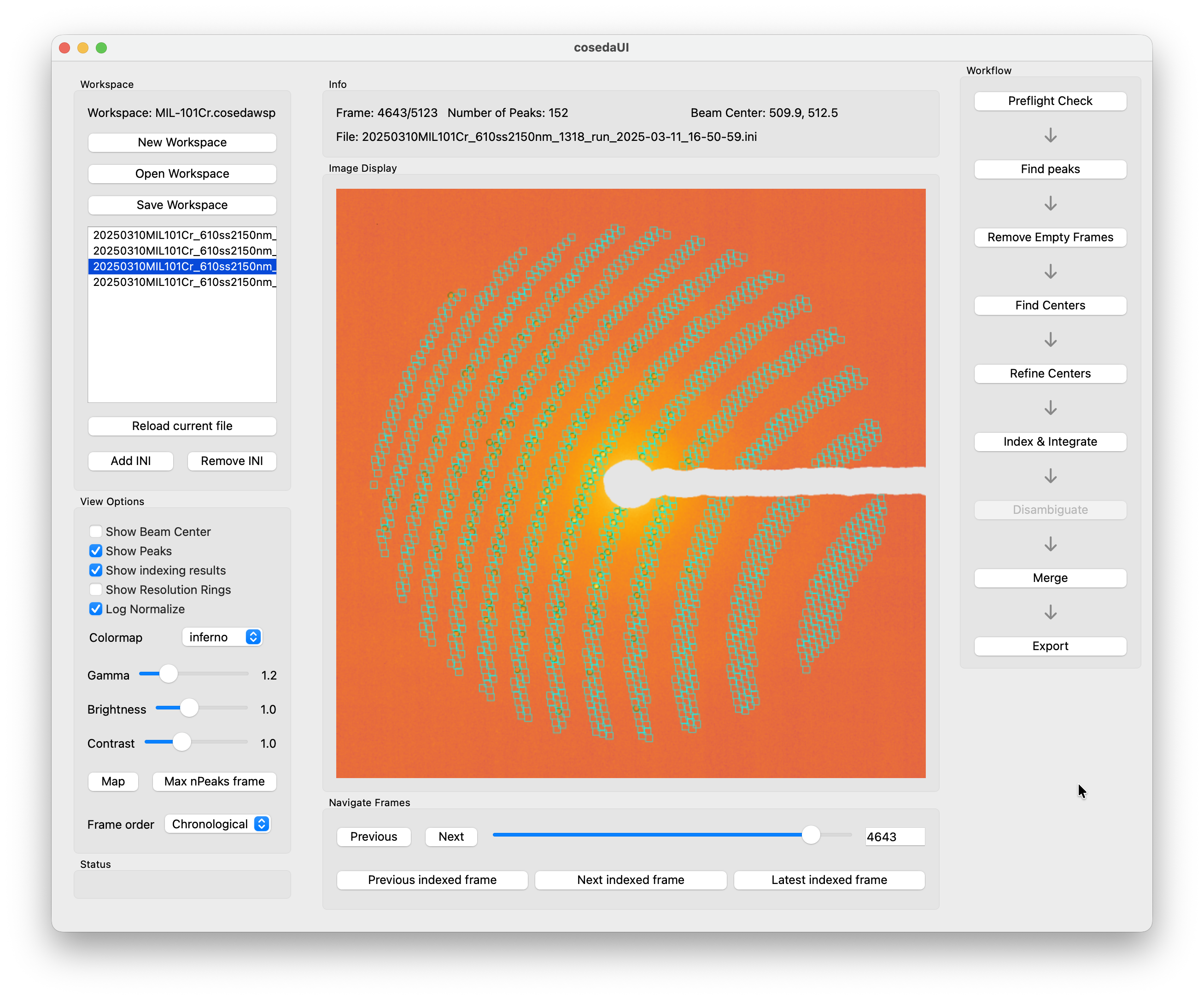
Once you click an indexing run in the tree, the Show indexing results tickbox in the view options of the main window will become active. You can toggle it, together with the Show peaks option to visually check if your indexing results are sensible.

After indexing is complete, open Tools → Workspace unit cell fit to inspect the distribution of indexed unit cell parameters. COSEDA scans all datasets in the workspace for their latest stream file and shows six histograms — one for each of a, b, c, α, β, γ. Sharp, symmetric peaks around the expected values suggest that the majority of patterns were indexed correctly. For this dataset, all three axes should converge tightly around 89.3 Å and all angles at 90°.

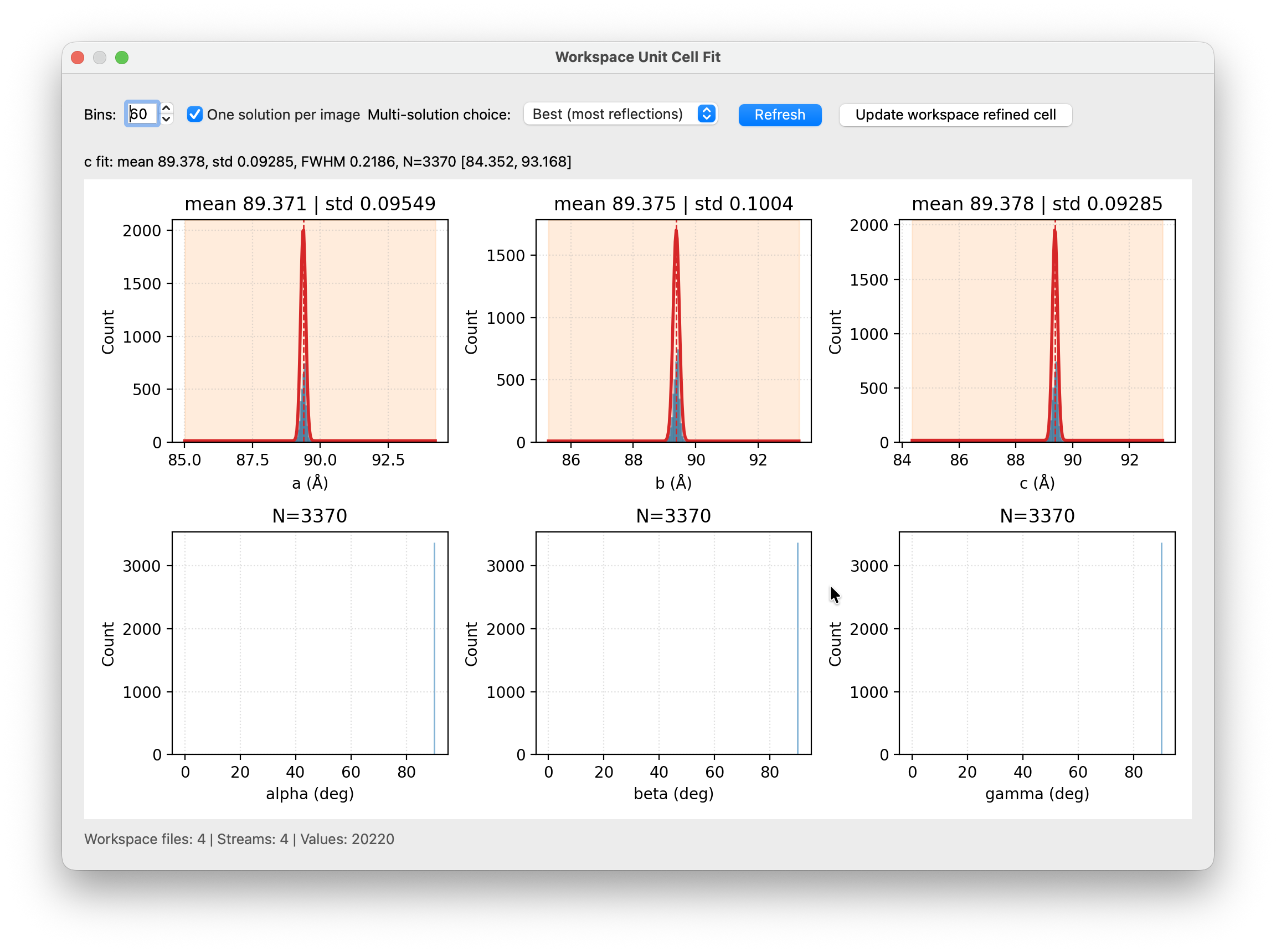
You can also use this tool to refine your cell estimate. Click and drag horizontally across the peak of interest in any histogram to fit a Gaussian. The fit result (mean, std, FWHM, N) appears above the plot. Once all six parameters look good, you can click Update workspace refined cell to write the fitted means back to the workspace file. The refined cell is then available in the Merge window as an improved reference for statistics. It can also feed directly back into a second indexing run. Update the cell in the Cell Editor with the refined parameters, tighten the XGandalf tolerance, and re-index. The tighter tolerance will reject more outliers and can improve your final indexing rate and data quality.

Merge

Open the Merge window. In the Select Run tab, choose the indexing run from the dropdown and click Combine → to concatenate all stream files into a single combined stream.

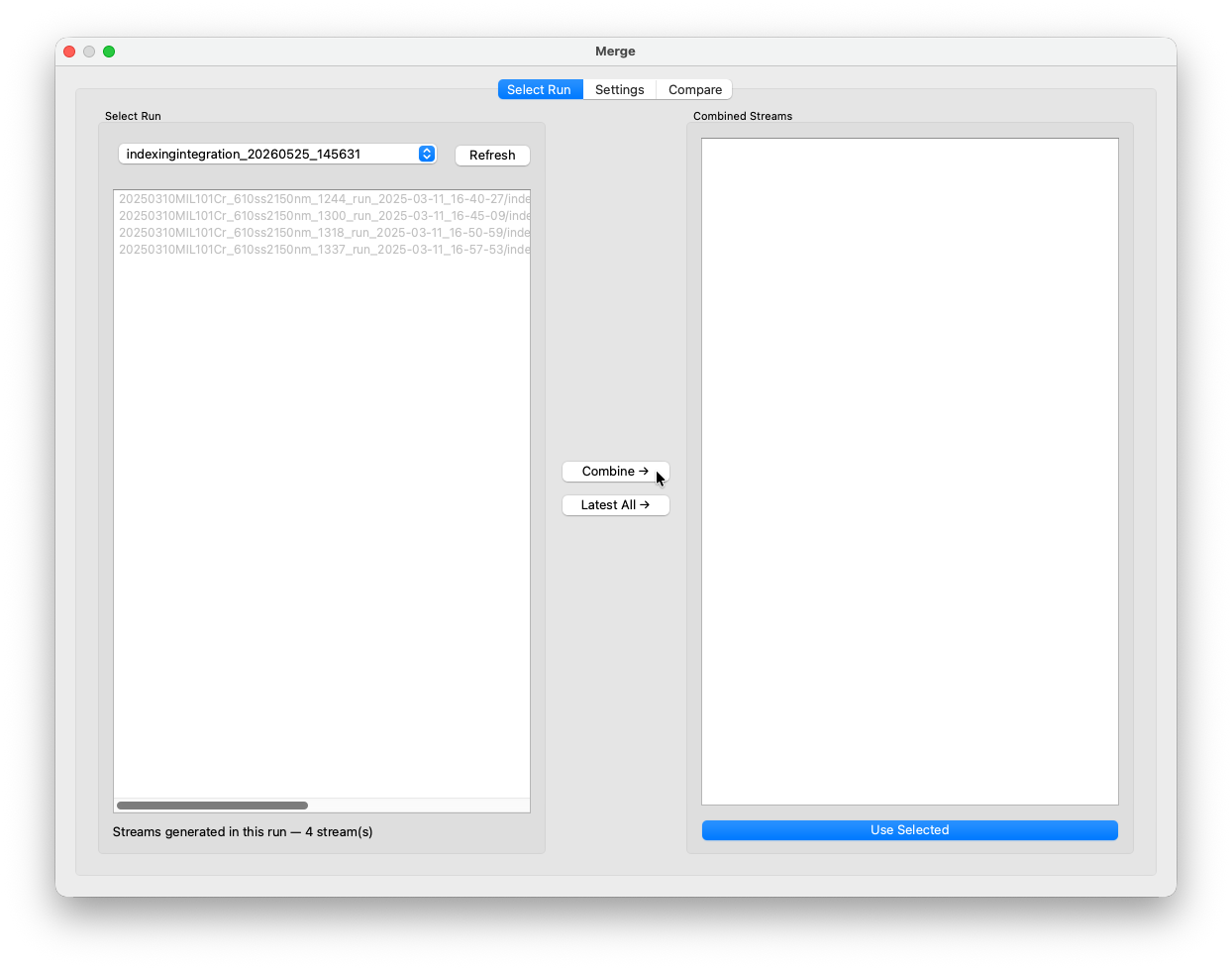
Switch to the Settings tab and fill in the parameters before clicking Merge.

Point Group

The symmetry Partialator uses when deciding which reflections are equivalent. Getting this wrong will not crash the merge but will silently produce incorrect statistics, so double-check before you start. For MIL-101(Cr) in space group F d -3 m, set it to m-3m.

Unique Axis

Only relevant for symmetries where a unique axis needs to be specified. CrystFEL expects this as part of the point group, e.g. 2/m_uab, and COSEDA adds this suffix for you when you select a unique axis here. Leave empty for cubic, orthorhombic or hexagonal symmetry.

Threads

Number of parallel CPU threads. Defaults to the number of available cores on your machine. Don’t go beyond that.

Min Resolution

A low-resolution cutoff in Å. Crystals with no reflections beyond this threshold are excluded from the merge entirely. The default is 5 Å, which is a reasonable sanity filter. A crystal that contributes nothing beyond 5 Å is unlikely to be a well-diffracting hit. Tick the ∞ checkbox to disable the cutoff and include all crystals regardless.

Iterations

Number of Partialator scaling and merging cycles. In each cycle Partialator refines per-crystal scale factors and rejects outlier crystals. 25 is usually sufficient. If the CC½ in the Merging sub-tab is still visibly climbing when the run finishes, increase this value and re-merge.

Model

The partiality model Partialator uses to account for the fact that each crystal only rotates through a limited angular range and therefore records only a fraction of each reflection’s full intensity. The options are offset, xsphere, unity, and ggpm. For electron diffraction, offset is the recommended default. The unity model assumes no partiality correction at all (every reflection is treated as fully recorded). It can be useful as a quick sanity check.

Min Measurements

Minimum number of independent observations a unique reflection must have to be included in the merged dataset. Reflections observed fewer times than this are discarded. The default of 5 is on the conservative side. It avoids including poorly sampled reflections but may reduce completeness in the outermost shells. Reduce it to 2 or 3 if your dataset is small and completeness matters more than noise.

Max ADU

Saturation cutoff. Peaks with a maximum pixel value above this threshold are excluded. By default set to ∞ (no cutoff). If your detector has a known saturation level, set this to reject saturated peaks that would otherwise distort the merged intensities.

Push Resolution

Extend merging beyond the apparent resolution of the data (in 1/nm), analogous to the same setting in indexamajig. Leave at 0 unless you have a specific reason to push further.

Use B-scaling

When checked, Partialator applies a per-crystal B-factor (temperature factor) correction on top of the overall scale factor. This can help when crystals in the dataset have systematically different resolution falloffs, but it adds an additional free parameter per crystal. For electron diffraction it is off by default and rarely needed. Leave it unchecked unless you have a reason to suspect systematic B-factor variation.

Output Every Cycle

When checked (default), Partialator writes an intermediate HKL file after each cycle. This is required for the split-half statistics tab to populate. Leave it on.

Once you are happy with the settings, click Merge.

Merging sub-tab

The Merging sub-tab updates live after each Partialator cycle.

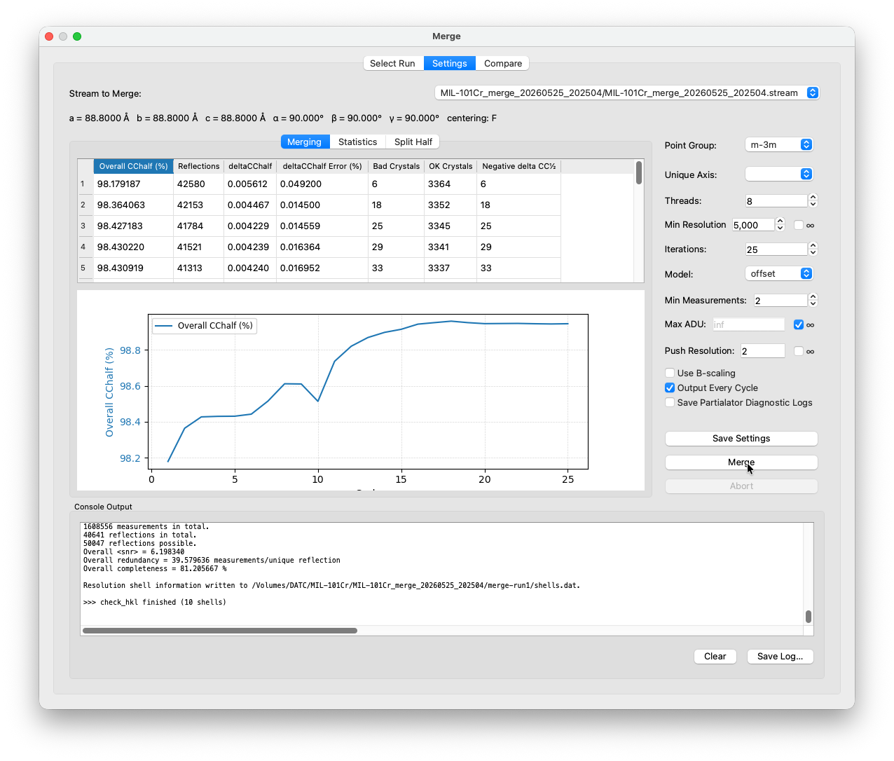
The key column to watch is Overall CC½. CC½ is the Pearson correlation coefficient between two randomly-split halves of the dataset, each merged independently. It measures self-consistency: if both halves agree well, the value is close to 1 (or 100%). A steadily rising CC½ that eventually flattens out is what you want to see. Once it stops improving from cycle to cycle, the merge has converged. If it is still noticeably climbing after 25 cycles, increase the iteration count in the settings and re-merge.

The ΔCC½ column shows the change in CC½ from the previous cycle. Partialator uses this as a per-crystal quality signal: any crystal whose inclusion reduces the overall CC½ (negative ΔCC½) gets flagged in Bad Crystals and removed. This is normal as a fraction of crystals in any SerialED dataset will be misindexed or too weak to contribute signal. As the merge converges, the Bad Crystals count should drop to near zero. A persistently high rejection count is a sign that something is off upstream, such as incorrect indexing or a wrong point group.

Statistics sub-tab

Once merging finishes, the Statistics sub-tab is populated by check_hkl with resolution-shell statistics.

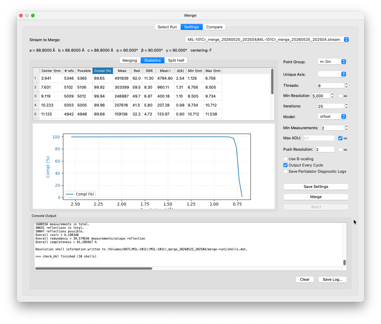
The columns to pay attention to:

• Completeness (%): the fraction of theoretically possible unique reflections that were actually measured at least once in that resolution shell. Aim for >90% in all shells you plan to use for structure solution. Low completeness in the outer shells usually means you are pushing the resolution too far.

• Redundancy (Red): the average number of times each unique reflection was measured across all crystals. High redundancy is one of the main advantages of serial crystallography. It reduces the effect of measurement noise through averaging. Values of 10–30× are typical and healthy. Suspiciously low redundancy (<5×) in the inner shells can may indicate a completeness problem or too few crystals indexed.

• SNR (Mean I/σ): the average signal-to-noise ratio per shell. High in the inner shells (often >10 for well-diffracting crystals), declining towards the resolution limit. The outer-shell SNR is one common way to decide where to cut your data — a commonly used threshold is SNR ≈ 2, below which the measurement noise dominates.

Split Half sub-tab

The Split Half sub-tab shows per-shell statistics using CrystFEL’s compare_hkl, comparing the two independently merged half-datasets.

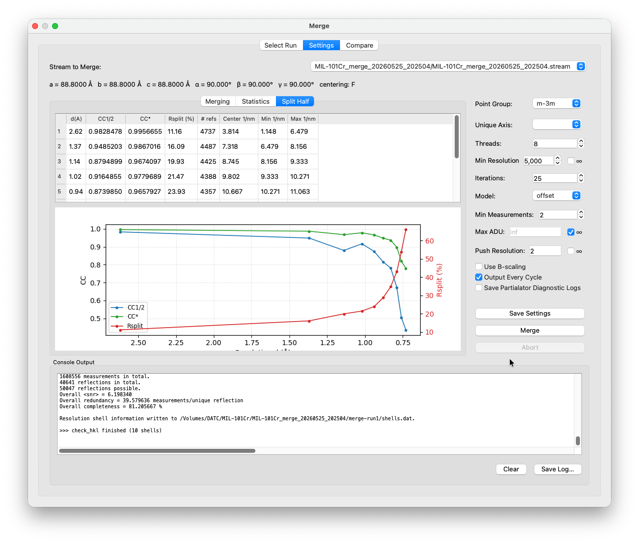
• CC½: the same Pearson correlation as above, but now broken down per resolution shell rather than as a single overall number. The inner shells should be close to 1. The outer shells will drop. The conventional cutoff for including a shell is CC½ > 0.3, below which the signal is dominated by noise.

• CC*: derived from CC½ as \(\text{CC}^* = \sqrt{\frac{2 \cdot \text{CC}_{1/2}}{1 + \text{CC}_{1/2}}}\). It estimates the true correlation between your merged data and a hypothetical perfect reference. This is less pessimistic than CC½ for high-resolution shells. CC* is commonly used together with CC½ to judge the resolution limit.

• Rsplit: defined as \(R_\text{split} = \frac{\sqrt{2} \sum |I_1 - I_2|}{\frac{1}{2} \sum (I_1 + I_2)}\), where \(I_1\) and \(I_2\) are the two half-dataset intensities. It is the serial-crystallography analogue of Rmerge and measures internal consistency: lower is better. As a rough estimate for SerialED data, values around 20–40% in mid-resolution shells are typical. Anything below 20% in the inner shells is good. Values consistently above 60% suggest a problem.

Export

Open the Export window from the toolbar. Finished merege runs should appear in the seclection box. Select the merge run from the list. The unit cell parameters are parsed automatically from the combined stream. Enter the space group (F d -3 m), (rough)chemical composition, and an optional resolution cutoff. Click Export HKLF4 to write the reflection file for SHELX, or Write INS to generate a ready-to-use instruction file.

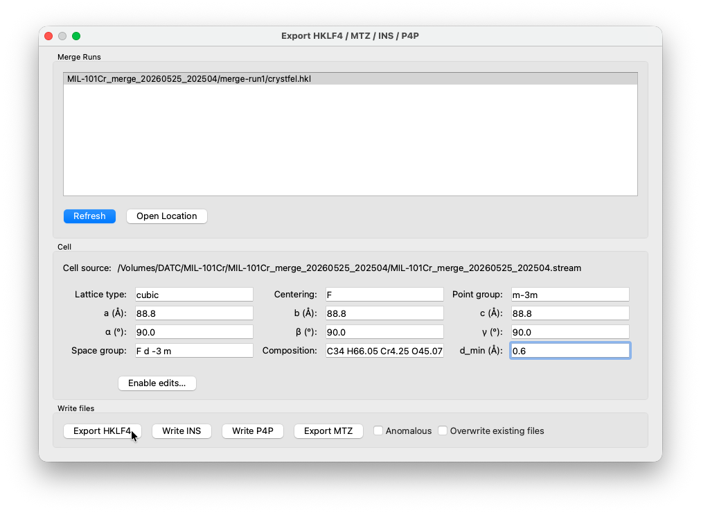
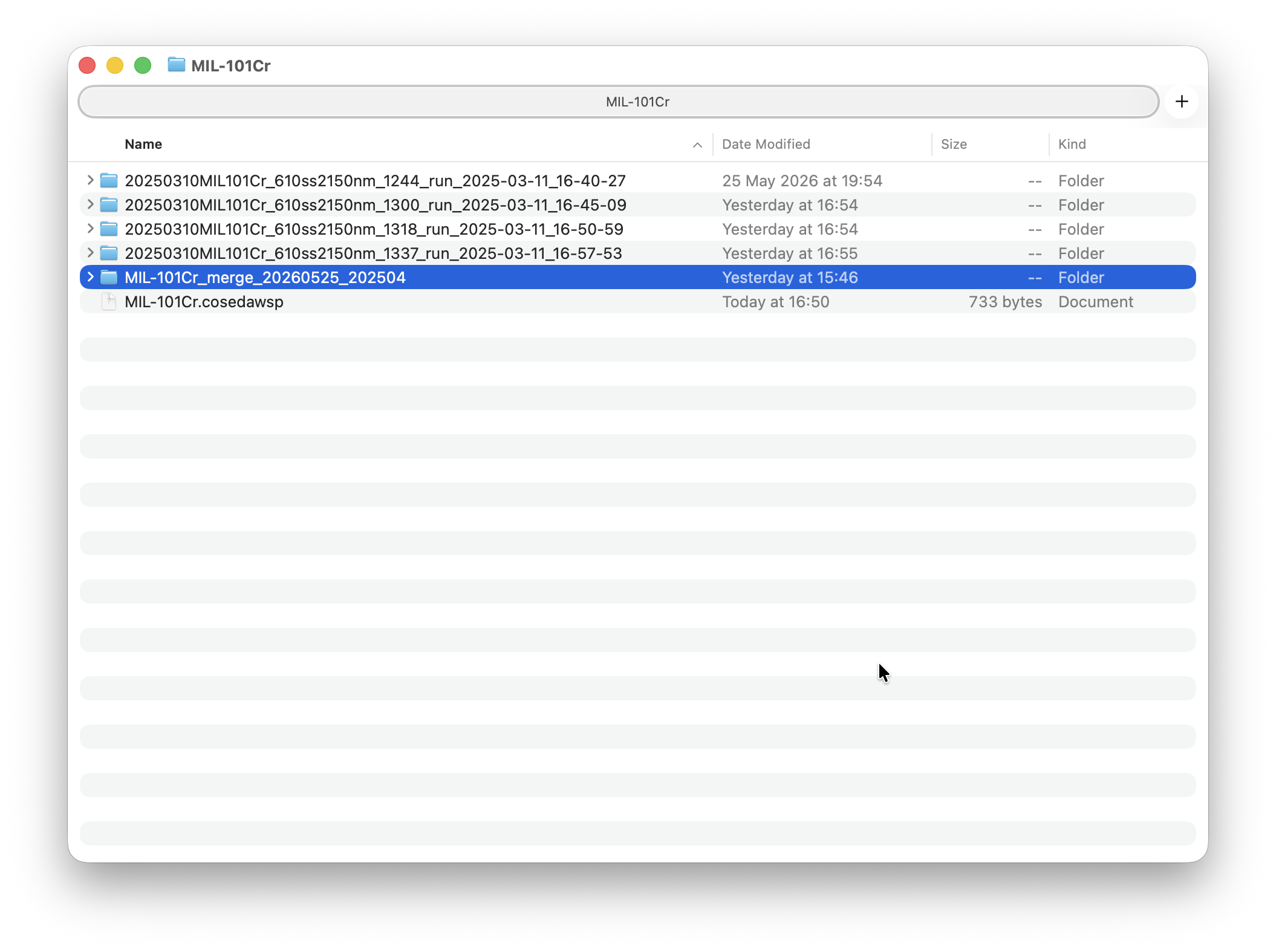
The exported files are written to the merge folder. You can click Open Location to open it directly in the file browser.

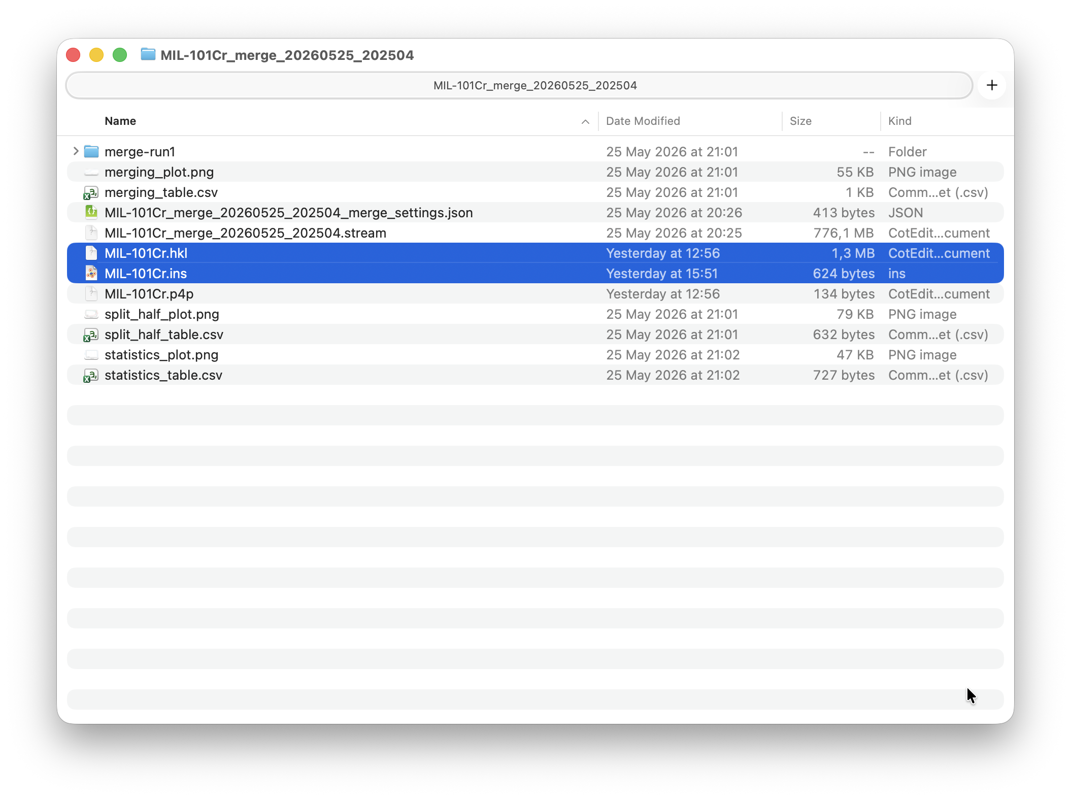
That’s it! Your MIL-101(Cr) dataset is processed and ready for structure solution. Take the .ins and .hkl files and proceed to Olex2 or the software of your choice.